Strategies I: Equities and Futures · Strategies
24Positioning and Sentiment
Every Friday at 3:30 in the afternoon, New York time, the CFTC publishes who held what in each futures market on the Tuesday before: producers and merchants, swap dealers, managed money. The report is public, cheap and old by the time it appears, and it has been studied for as long as it has existed. De Roon, Nijman and Veld found that hedgers’ positions help explain futures returns across twenty markets: speculators who take the other side of hedging demand are paid for it. On this chapter’s synthetic commodities, where that payment is planted, the hedgers’ position has a rank IC of 0.044 with the next week’s returns when it is known at once, 0.038 when it is known on Friday, and 0.017 three weeks later. On nine years of real corn positioning, the most studied signal in the market is not significant. The build is firm.posisig.
24.1 Positioning reports
As of September 2026 — The Commitments of Traders schedule
The CFTC’s Commitments of Traders report is generally published each Friday at 3:30 pm Eastern Time with positions as of the immediately preceding Tuesday; the Commission says it takes three days to process the data, and holidays shift the schedule, which it publishes in advance. Book 3, chapter 9 describes the report’s trader categories.
Definition 24.1 (Hedging pressure, positioning signal)
Hedging pressure is the net position of hedgers in a futures market, usually net short for producers, as a share of open interest; speculators who take the other side earn a risk premium that rises with it. A positioning signal is a trading signal built from reported positions of a category of traders, as known at the time of the trade.
The record is older than the chapter’s other signals. Bessembinder found that returns in currency and agricultural futures vary with hedgers’ net holdings after controlling for systematic risk; de Roon and co-authors found that both a market’s own hedging pressure and that of related markets in its group affect returns, and that the effect survives a control for price pressure. The logic is the insurance view of futures: hedgers pay to lay off risk, and whoever carries it is paid.
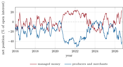
In real positions the two sides are mirror images. In the CFTC’s disaggregated data for CBOT corn, 2016 to 2026, managed money’s net position ranged from to of open interest, and its correlation with the producers’ and merchants’ net position is (Figure 24.1): speculators absorb what hedgers lay off.
s1_posisig.corn.Does corn’s managed money position predict corn’s price? The test uses the position’s 52-week z-score as published by each month’s end and the IMF maize price’s change over the month after next (monthly averages; skipping a month keeps the signal’s own month out of the return). Over 113 months, 2017 to 2026, the correlation is 0.098 (). After record-long positions (z-score above 1) the next three months’ price change averaged (28 cases), after record-short ones (24), and otherwise (59): if anything, speculators’ extremes were followed by moves in their favour, as the hedging-pressure view would have it, but with a hundred months the evidence says nothing either way.
24.2 The value of a report, and its age
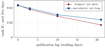
firm.posisig plants the mechanism in firm.synthfut’s ten commodities (Listing 24.1). Hedgers’ net short position follows an AR(1) with a half-life of 20 trading days, in standard deviations; it adds a premium of 0.3 times the market’s volatility a year per standard deviation to the next day’s return. Speculators’ reported net long position is the hedging pressure plus half a standard deviation per unit of their own 60-day trend, plus noise. Positions are measured on the fifth day of each week (the “Tuesday”) and known after a publication lag. The signal is measured every day against the next five days’ returns, across the ten markets.
| publication lag (trading days) | 0 | 3 (Friday) | 10 | 21 |
|---|---|---|---|---|
| hedgers’ position: rank IC | 0.044 | 0.038 | 0.029 | 0.017 |
| t-statistic | 5.1 | 4.4 | 3.4 | 2.0 |
| speculators’ position: rank IC | 0.043 | 0.039 | 0.031 | 0.024 |
The Tuesday-to-Friday lag costs 14% of the signal (Figure 24.2); three weeks cost 62%. Both follow from the pressure’s persistence: with a half-life of 20 days, three days of age keep 90% of it, 21 days 48%. The speculators’ position loses its value more slowly because part of it is trend-chasing, and firm.synthfut’s planted trends are slow: the trend component of the signal ages well even though it has nothing to do with hedging.
s1_posisig.lag_table.The contrarian rule, selling when speculators are at a record long, fails in the model by construction: after a 52-week z-score above 1.5 the next quarter’s return averaged annual volatilities, after one below it averaged , and otherwise. A contrarian rule needs a mechanism in which speculators are the ones paying, crowding into positions that later unwind; the model has none, and neither the corn data nor the sources fetched for this chapter supply one.
24.3 Surveys and sentiment indices
Definition 24.2 (Sentiment index)
A sentiment index summarises investors’ optimism or pessimism from surveys or market-based proxies (issuance, fund flows, first-day returns of new issues, valuation spreads), usually as the first principal component of several proxies.
Baker and Wurgler showed what sentiment predicts in the cross-section of stocks: when sentiment is low at the start of a period, the stocks hardest to value and to arbitrage (small, young, volatile, unprofitable, non-dividend-paying, extreme growth and distressed stocks) earn relatively high returns later; when it is high, they earn relatively low ones. Sentiment is a conditioning variable more than a signal: it says which stocks a wave of optimism has moved furthest from value, and when their mispricing is likely to be large. It changes slowly and is published with a lag, so its age matters less than a weekly positioning report’s.
Options positioning is the third source: put–call ratios, open interest by strike and dealers’ likely gamma. Chapter 15 measured what informed option demand says about stocks; chapter 13 measured what dealers’ hedging does near the close. As positioning, options add the view of the traders who pay for convexity, reported daily and by strike.
24.4 Strategy files
Strategy file 24.1 — Hedging-pressure signal
Who pays you, and why. Hedgers who pay a premium to lay off price risk.
Instruments and venues. Commodity and financial futures with COT reporting.
Signal. Hedgers’ net short position as a share of open interest, as published (Friday), within market or across a group.
Sizing and execution. Long markets with high hedging pressure, short low; weekly, volatility-scaled.
Costs. Low; weekly rebalancing.
How it dies. More speculative capital competing to absorb hedging; changing hedging programmes.
Horizon, capacity, infrastructure. Weeks; the COT archive with release dates.
Backtest honestly. Positions only from the Friday of each report (later after holidays), never from Tuesday.
Sources. Bessembinder (1992); de Roon, Nijman and Veld (2000); this chapter: IC 0.038 as published, synthetic.
Strategy file 24.2 — Extreme-positioning contrarian
Who pays you, and why. Only if speculators crowd into positions and unwind them together; otherwise nobody.
Instruments and venues. Futures with COT reporting.
Signal. Managed money’s net position at a multi-year extreme.
Sizing and execution. Fade the extreme, small, with a stop.
Costs. Low.
How it dies. It may not live: in corn, 2017–2026, extremes were followed by moves in the speculators’ favour.
Horizon, capacity, infrastructure. Months.
Backtest honestly. Extremes as measured with past data only; published dates; enough extremes to test.
Sources. No supporting result verified; this chapter’s corn test ( for the opposite sign).
Strategy file 24.3 — Options-positioning signal
Who pays you, and why. Traders who pay for protection or leverage, whose demand is visible in option volumes and open interest.
Instruments and venues. Stocks and indices with listed options.
Signal. Put–call ratios and open interest by strike, conditioned on sentiment.
Sizing and execution. Tilts in stock or index positions; daily.
Costs. Moderate.
How it dies. Hedging flow that looks like speculation; crowding.
Horizon, capacity, infrastructure. Days to weeks; options data by strike.
Backtest honestly. Open interest as reported the next morning; volumes signed only if the data allow.
Sources. Chapter 15; Baker and Wurgler (2006) for sentiment as a conditioning variable.
24.5 Tutorial: record long
Goal. Plant hedging pressure in synthetic commodities, measure what the positioning signal is worth at each publication lag and at extremes, and test the real corn positioning series. End state: the table and the two figures.
Reports and the market: the publication schedule and the planted hedging pressure.
def published(x, every: int = 5, offset: int = 1, lag: int = 3):
    x = np.asarray(x, float)
    T = len(x)
    out = np.full(x.shape, np.nan)
    last = None
    report_days = set(range(offset, T, every))
    pending = []
    for t in range(T):
        if t in report_days:
            pending.append((t + lag, x[t].copy()))
        while pending and pending[0][0] <= t:
            last = pending.pop(0)[1]
        if last is not None:
            out[t] = last
    return out


def hedging_market(r, vol, half_life: float = 20.0, premium: float = 0.3, chase: float = 0.5, noise: float = 0.5,
                   rng=None):
    rng = rng or np.random.default_rng(24)
    r = np.asarray(r, float)
    T, N = r.shape
    phi = math.exp(-math.log(2) / half_life)
    h = np.zeros((T, N))
    for t in range(1, T):
        h[t] = phi * h[t - 1] + math.sqrt(1 - phi**2) * rng.standard_normal(N)
    out = r.copy()
    out[1:] += premium * np.asarray(vol) * h[:-1] / 252.0          # hedgers short -> speculators long earn the premium
    c = np.cumsum(out, axis=0)
    trend = np.zeros((T, N))
    trend[60:] = (c[60:] - c[:-60]) / (np.asarray(vol) * math.sqrt(60 / 252))
    spec = h + chase * trend + noise * rng.standard_normal((T, N))
    return {"r": out, "hedge": h, "spec": spec}
Listing 24.1. The reporting schedule and a market with hedging pressure. code/firm/posisig/firm_posisig.py Real corn: managed money’s z-score as published by month-end against maize prices.
def corn():
    with open(DATA / "cot_corn_disagg.csv") as fh:
        rows = list(csv.DictReader(fh))
    d = [dt.date.fromisoformat(r["date"]) for r in rows]
    pos = [{k: int(v) for k, v in r.items() if k != "date"} for r in rows]
    mm = np.array([net_share(p, "mm") for p in pos])
    pm = np.array([net_share(p, "pm") for p in pos])
    z = zscore(mm, 52)
    with open(DATA / "ags_monthly.csv") as fh:
        ag = list(csv.DictReader(fh))
    px = np.log(np.array([float(a["maize"]) for a in ag]))
    xs, ys, q = [], [], []
    for k, a in enumerate(ag[:-2]):
        y, mo = int(a["month"][:4]), int(a["month"][5:])
        end = dt.date(y, mo, calendar.monthrange(y, mo)[1])
        known = [i for i in range(len(d)) if d[i] + dt.timedelta(days=3) <= end]   # released by Friday
        if not known or np.isnan(z[known[-1]]):
            continue
        xs.append(z[known[-1]])
        ys.append(px[k + 2] - px[k + 1])
        if k + 4 < len(px):
            q.append((z[known[-1]], px[k + 4] - px[k + 1]))
    xs, ys, q = np.array(xs), np.array(ys), np.array(q)
    c = float(np.corrcoef(xs, ys)[0, 1])
    grp = {n: (float(q[m, 1].mean()), int(m.sum())) for n, m in
           (("high", q[:, 0] > 1), ("low", q[:, 0] < -1), ("middle", np.abs(q[:, 0]) <= 1))}
    return {"n": len(xs), "corr": c, "t": c * math.sqrt(len(xs)), "groups": grp,
            "mm_pm_corr": float(np.corrcoef(mm, pm)[0, 1]), "mm_range": (float(mm.min()), float(mm.max())),
            "dates": d, "mm": mm, "pm": pm}
Listing 24.2. Corn positioning against the maize price. code/strategies-1/24-positioning-and-sentiment/python/s1_posisig.py - Run
lag_table(),extremes()andcorn(), andfig_posisig.py.
What to change next. Plant a crowding mechanism (speculators’ positions pushing prices, which revert) and see the contrarian rule appear; shorten the pressure’s half-life to five days and measure the Friday lag’s cost; add swap dealers as a third category.
24.6 Build: positioning signals
Purpose. Reports as known on each day, a market with hedging pressure, forward returns, rank ICs and z-scores.
Interface. published(x, every, offset, lag), hedging_market(r, vol, half_life, premium, chase, noise, rng), forward(r, h), ic(signal, fwd, step, overlap), zscore(x, window); firm.cot’s net_share for real reports.
Rules. A report is usable only from its publication day; ICs with overlapping horizons have their t-statistics corrected.
Acceptance tests. code/firm/posisig/tests/: a Tuesday-to-Friday schedule by hand, forward sums, IC and its overlap correction, the premium as planted.
Stretch. The CFTC’s actual release calendar with holiday shifts; cross-market hedging pressure within groups; a crowding mechanism.
Sources and further reading
- F. A. de Roon, T. E. Nijman and C. Veld, “Hedging pressure effects in futures markets”, Journal of Finance 55(3), 2000.
- H. Bessembinder, “Systematic risk, hedging pressure, and risk premiums in futures markets”, Review of Financial Studies 5(4), 1992.
- M. Baker and J. Wurgler, “Investor sentiment and the cross-section of stock returns”, Journal of Finance 61(4), 2006.
- US Commodity Futures Trading Commission, Commitments of Traders (release schedule and disaggregated reports); IMF, global price of maize (via FRED).
24.7 Exercises
Exercise 24.1 ★
A position measured on Tuesday is published on Friday. On which day can a backtest first use it, and what does using it on Tuesday do to the results?
Solution
Solution of Exercise 24.1.
From Friday’s close (after the 3:30 pm release), or Monday’s open to be safe; later in holiday weeks. Using it on Tuesday gives the backtest three days of information nobody had, and credits it with the signal’s freshest, most valuable part.
Exercise 24.2 ★
Hedging pressure follows an AR(1) with a half-life of 20 trading days. What share of it survives three days? Ten? Twenty-one?
Solution
Solution of Exercise 24.2.
: , , . The measured ICs fall a little faster (to 86%, 66% and 38% of the immediate one) because a report is used for five days after it becomes known.
Exercise 24.3 ★
Why are managed money’s and producers’ positions in corn almost perfect mirror images?
Solution
Solution of Exercise 24.3.
Every futures contract has a long and a short. The report’s categories cover almost all open interest, and in corn the two largest net positions are hedgers’ (producers and merchants, net short) and speculators’ (managed money): when one adds, the other takes the other side.
Exercise 24.4 ★★
With 113 months, how large must a correlation be to be significant at 5%? Is corn’s 0.098?
Solution
Solution of Exercise 24.4.
About . Corn’s 0.098 is about half of that ().
Exercise 24.5 ★★
Why does the speculators’ signal keep more of its value than the hedgers’ at long lags?
Solution
Solution of Exercise 24.5.
Part of the speculators’ position is trend-chasing, and firm.synthfut’s planted trends have a half-life of a year: that part of the signal predicts returns for longer than the hedging pressure, whose half-life is 20 days.
Exercise 24.6 ★★
Why does the contrarian rule fail in the model, and what would have to be planted for it to work?
Solution
Solution of Exercise 24.6.
In the model speculators are paid for absorbing hedging, so large speculative longs come with high expected returns: fading them loses. A contrarian rule needs speculators to be the ones paying: positions that push prices away from value and later unwind, a crowding mechanism the model does not have.
Exercise 24.7 ★★★
Coding. Run lag_table(5.0), with a half-life of five days instead of twenty. How much of the hedgers’ IC does the Friday lag cost now?
Solution
Solution of Exercise 24.7.
The IC falls from 0.032 known at once to 0.019 known on Friday: the lag costs 42% of the signal, against 14% with a half-life of twenty days. The shorter the pressure lasts, the more a three-day delay costs.
Exercise 24.8 ★★★
Find the flaw. “We built a sentiment index from surveys and it predicted the market’s next-month return with over 1990–2020, using the survey values as dated.”
Solution
Solution of Exercise 24.8.
Survey values dated by their reference period, not by their publication, give the backtest information before it was public; indices built with principal components over the whole sample use later data to weight earlier values; and the proxies were chosen after the fact. Use publication dates and an index rebuilt with data available at each date.
24.8 Problem: Record Long
Problem 24.1
Weekend problem — a report’s value and its age
The chapter’s synthetic commodities, the corn reports and the public record.
Part I — Reports.
- When is the COT report published, and for which day?
- Define hedging pressure and a positioning signal.
- What did Bessembinder and de Roon, Nijman and Veld find?
- How do corn’s managed money and producers’ positions relate?
Part II — Corn.
- Describe the corn test and why it skips a month.
- Give its correlation and t-statistic.
- What followed record longs and record shorts?
- What does a hundred months allow you to conclude?
Part III — The model.
- Describe the planted hedging pressure and the speculators’ position.
- Give the hedgers’ IC at each publication lag.
- Explain the Friday lag’s cost from the half-life.
- Why does the contrarian rule fail here?
Part IV — The verdict.
- State the named result: the IC of the positioning signal and the effect of the Tuesday-to-Friday publication lag.
- Define a sentiment index; what did Baker and Wurgler find?
- How is sentiment used differently from positioning?
- What does options positioning add?
- How would you backtest a COT strategy honestly?
- Which strategy file lacks a mechanism?
- How does this chapter relate to chapter 20’s carry?
- In one sentence: who pays a positioning trader?
Solution
Solution of Problem 24.1.
- Generally Friday at 3:30 pm Eastern Time, for the preceding Tuesday.
- Hedgers’ net position as a share of open interest; a signal from reported positions as known at the time.
- Returns in currency and agricultural futures vary with hedgers’ net holdings; own and within-group hedging pressure affect returns in 20 markets.
- As mirror images: a correlation of .
- Managed money’s 52-week z-score at each month-end against the maize price’s change over the month after next, so that the signal’s month does not overlap the return.
- 0.098, .
- over three months after record longs, after record shorts, otherwise.
- Nothing either way.
- An AR(1) with a half-life of 20 days earning 0.3 volatilities a year per standard deviation; speculators hold it plus trend-chasing and noise.
- 0.044, 0.038, 0.029 and 0.017 at lags of 0, 3, 10 and 21 days.
- Three days keep of the pressure; a report used for five days loses a little more: 14%.
- Speculators are paid in the model, so their extremes come with high expected returns.
- Named result. The hedgers’ positioning signal has a rank IC of 0.044 with the next five days’ returns when known at once and 0.038 when published three days later (14% less), falling to 0.017 at 21 days; the speculators’ signal, 0.043 and 0.039.
- A summary of investors’ optimism from surveys or market proxies; low sentiment is followed by relatively high returns on hard-to-value stocks.
- As a slow conditioning variable, saying which stocks are most mispriced, not as a weekly trading signal.
- The positions of those paying for convexity, daily and by strike.
- Reports only from their publication date, holiday shifts included, and costs.
- The extreme-positioning contrarian.
- Both pay whoever carries risk that others want to lay off: carry through the curve, hedging pressure through positions.
- Hedgers who pay to lay off price risk.
24.9 Interview questions
Interview question 24.1 ★ researcher
What does the Commitments of Traders report contain, and what can it not tell you?
Solution
Solution of Interview question 24.1.
Open interest and the long and short positions of reportable trader categories (producers and merchants, swap dealers, managed money, others), weekly for Tuesday; it cannot tell you positions within the week, positions in other markets or over the counter, or why a category trades.
Interview question 24.2 ★★ researcher
Why might speculators earn a premium in futures markets?
Solution
Solution of Interview question 24.2.
Hedgers pay to transfer price risk: producers selling futures below the expected spot price leave a premium for the speculators who buy them.
Interview question 24.3 ★★ trader
Managed money is at a record long in crude oil. What do you do?
Solution
Solution of Interview question 24.3.
A record long alone is not a signal: check whether it is absorbing hedging (producers’ positions, curve shape, inventories) or crowding on a trend; check the evidence for that market; size any fade small, because extremes can persist and in some data are followed by further gains.
Interview question 24.4 ★★ developer
How would you store COT data so that backtests use each report only when it was public?
Solution
Solution of Interview question 24.4.
Each report with its as-of date (Tuesday) and its publication timestamp, from the CFTC’s release calendar; revisions kept as new versions; queries always by publication time.
Interview question 24.5 ★★ researcher
How would you build a sentiment index, and how would you test it?
Solution
Solution of Interview question 24.5.
Choose proxies with a reason (surveys, issuance, flows, new-issue returns), orthogonalise them to macroeconomic conditions, combine them with weights estimated only on past data, and test the index on the cross-section of hard-to-value stocks out of sample.
Interview question 24.6 ★★★ researcher
A signal is an AR(1) with coefficient per day and predicts the next day’s return with correlation . Derive its correlation with the return days after it was measured, and the average correlation for a report used over the five days after a lag of days.
Solution
Solution of Interview question 24.6.
With , and , so the correlation of with is . A report used on days has average correlation .