Strategies I: Equities and Futures · Strategies

2Short-Term Reversal

Buy yesterday’s losers and sell yesterday’s winners. On the synthetic market the residual version of this rule has a rank information coefficient of 0.041 against the next day’s return, and the naive book built from it (gross exposure one, rebuilt at every close, in the 500 most liquid names) has a Sharpe ratio of 13.0 before costs. At ten basis points per unit traded it is $-3.4$ . The strategy is real (it is one of the oldest anomalies in the literature, and the synthetic market plants it) and nearly untradeable as written, because it turns over three quarters of its book every day. This chapter is about the one-day reversal and its variants, and above all about how it is traded: with costs inside the optimiser it earns a Sharpe ratio of 1.7 after costs at $100 million and about nothing at $1 billion. The build is firm.reversal.

2.1 Why prices reverse: paying for immediacy

Definition 2.1 (Short-term reversal)

Short-term reversal is the tendency of stocks with low returns over a short past window (a day, a week, a month) to outperform, over the next such window, stocks with high returns; a short-term reversal strategy buys the recent losers and sells the recent winners.

The effect has been in the literature for as long as there have been return files. Jegadeesh found significant negative first-order serial correlation in monthly returns, the extreme deciles of a forecast built on it differing by 2.49% a month over 1934–1987; Lehmann found that one week’s winners and losers reverse sizeably the next week, with profits that survived corrections for bid–ask spreads and plausible costs. Lehmann’s reading has become the standard one: the reversal is “inefficiency in the market for liquidity around large price changes”. A trader who must sell now pushes the price down, the price comes back as others absorb the flow, and whoever bought from the hurried seller is paid for providing immediacy. Nagel made the interpretation explicit, treating reversal returns as a proxy for the returns from liquidity provision, and found them highest when liquidity is scarcest: expected returns and conditional Sharpe ratios spike in financial turmoil, predictably with the VIX.

Two consequences shape everything that follows. First, the part of a price move that is news should not reverse, and the part that is pressure should, so a good reversal signal tries to isolate pressure. Second, the reversal trader is a market maker at a daily horizon: the edge is the reward for trading, and the strategy lives or dies by the cost of that trading.

2.2 Daily reversal: raw, residual, industry-adjusted

Definition 2.2 (Residual reversal, industry-adjusted reversal)

Residual reversal is short-term reversal computed on residual returns, the part of each stock’s return that its factor exposures do not explain. Industry-adjusted reversal is reversal computed on each stock’s return in excess of its industry’s average return.

A stock’s day is the market’s day, its industry’s day and its own. The market and industry parts are shared by hundreds of stocks and largely reflect news about the economy; they are not what a hurried seller moves. The synthetic market (Book 7, chapter 5) plants a reversal of 5% of each day’s specific shock and nothing on the common parts, so the cleaner the signal’s estimate of the specific shock, the better it forecasts:

years 3 to 10	raw	industry	residual	truth
mean rank IC, all listed names	0.037	0.038	0.041	0.044
mean rank IC, 500 most liquid names	0.037	0.039	0.041	0.044
naive book: Sharpe ratio before costs	6.69	7.24	12.96
return a year; turnover a day	27.0%; 75%	28.2%; 75%	30.3%; 76%
Sharpe ratio after 10 bp	$-2.62$	$-2.46$	$-3.43$
break-even cost per unit traded	7.2 bp	7.5 bp	7.9 bp

(The naive books trade the 500 most liquid names; “industry” is the industry-adjusted signal and “truth” the planted expected return.) The information coefficient rises only from 0.037 to 0.041, but the residual book’s Sharpe ratio almost doubles, because the raw book carries industry and style exposures that add risk without return. Blitz, Huij, Lansdorp and Verbeek found the same on US data: conventional reversal strategies have dynamic exposures to the Fama–French factors, and the residual version, without them, earns risk-adjusted returns twice as large, significant net of trading costs even among large caps after 1990. Da, Liu and Schaumburg went further in the same direction, removing the part of the past return explained by cash-flow news (measured with analysts’ forecast revisions); their enhanced strategy’s risk-adjusted return was four times the standard one’s.

None of these gross numbers survives costs as a naive book. Every book in the table turns over about three quarters of its gross each day; at ten basis points per unit of weight traded it pays 38% a year against a gross return of 27–30%. The break-even cost, the gross return divided by twice the turnover (Book 7, chapter 16), is between 7 and 8 basis points for all three, and ten is already a low cost for a daily book (Book 7, chapter 16 made the same point with the raw signal).

2.3 Intraday and overnight reversal

Definition 2.3 (Overnight reversal)

Overnight reversal is the tendency of a stock’s overnight return, from the previous close to the open, to be partly reversed during the following trading session, and of its trading-session return to be partly reversed overnight; a strategy on it trades between the two parts of the day.

Splitting the day in two changes the picture. Lou, Polk and Skouras found strong continuation within each part (overnight returns predict overnight returns, and intraday returns intraday returns, for years) together with an offsetting cross-period reversal, and in fourteen strategies that profits were earned either entirely overnight or entirely intraday; for reversal, overnight. Akbas, Boehmer, Jiang and Koch counted, in each month, how often a positive overnight return was followed by a negative trading-day reversal, and found that stocks with more such days (a more intense “tug of war” between overnight and daytime clienteles) earned higher returns later. Inside the day, Heston, Korajczyk and Sadka traced the short-term reversal to temporary liquidity imbalances lasting less than an hour and to bid–ask bounce, next to a striking continuation at intervals that are exact multiples of a day.

firm.reversal computes the overnight and intraday signals from open and close prices (functions overnight and intraday); the synthetic market has no open, so the chapter measures only the daily variants, and the two strategy files on them rest on the published record.

2.4 Costs: where the strategy lives or dies

A daily reversal book needs three things the naive book does not have. A forecast in units of return, so that it can be compared with costs: Grinold’s rule (Book 7, chapter 15) gives $\alpha_i = \mathrm{IC}\,\sigma_i\,z_i$ , with $z_i$ the residual scaled by the stock’s own specific volatility and standardised across names, and the IC of 0.041 measured on year 2 only. A cost model: half a spread of 2 basis points plus square-root impact $0.7\,\sigma_i\sqrt{Q_i/V_i}$ (Book 7, chapter 27). And an optimiser that compares the two for every name every day. With a diagonal risk model the problem separates by name: each name’s trade is a closed-form step that shrinks the desired trade by the linear cost and damps it by the impact, and neutrality to the risk model’s fifteen factors adds one small system for the multipliers (Listing 2.1).

Residual reversal on all names, earnings days skipped:

fund size	$100m	$1bn	$10bn
costs ignored: Sharpe ratio before, after	16.92, $-27.8$	16.92, $-31.7$	16.92, $-32.2$
costs ignored: trading costs a year	246%	738%	2 293%
costs inside: Sharpe ratio before costs	8.42	3.97	1.72
costs inside: Sharpe ratio after costs	1.72	0.09	0.19
costs inside: gross, costs, net (% a year)	10.23, 8.18, 2.05	2.44, 2.38, 0.05	0.45, 0.40, 0.05
costs inside: turnover a day; gross	18.6%; 0.91	3.9%; 0.48	0.5%; 0.18
net profit a year	$2.0 million	$0.5 million	$4.8 million

The cost-blind book trades 186% of its capital a day at a gross exposure of 2.48: its gross Sharpe ratio of 16.9 is the best of any book in the chapter, and at $100 million it pays 246% of its capital a year in costs. With costs inside, the book at $100 million trades a tenth as much, keeps half its gross Sharpe ratio, and nets 1.72. At $1 billion it trades 3.9% a day and earns its costs and nothing more; at $10 billion it barely trades (Figure 2.1). The strategy’s edge per trade is its information coefficient times a day’s volatility, about sixteen basis points for a name two standard deviations out, and a square-root cost reaches that on a trade of 1% of the name’s daily volume. The capacity of a one-day reversal is therefore small: for this signal, somewhere between $100 million and $1 billion.

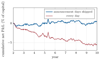
Residual reversal with costs inside the optimiser, on the synthetic market: Sharpe ratio before and after costs against fund size. Data: s1_reversal.traded. — **Figure 2.1.** Residual reversal with costs inside the optimiser, on the synthetic market: Sharpe ratio before and after costs against fund size. Data: `s1_reversal.traded`.

One more filter made the difference between a small loss and a small profit. The synthetic market plants a post-earnings drift (Book 7, chapter 11), and a stock that falls on bad earnings keeps drifting down: a reversal book that buys it is betting against news. Skipping names on their announcement day, which is scheduled and public, costs almost nothing in information coefficient (0.040 against 0.041) and turns the book at $1 billion from $-0.70\%$ a year (Sharpe ratio $-1.04$ ) to $+0.05\%$ (Figure 2.2). It is Da, Liu and Schaumburg’s point on a small scale: moves explained by fundamentals do not reverse.

The cost-aware reversal book at $1 billion, net of costs, with and without the earnings filter. Data: s1_reversal.traded. — **Figure 2.2.** The cost-aware reversal book at $1 billion, net of costs, with and without the earnings filter. Data: `s1_reversal.traded`.

2.5 The decline of reversal profits

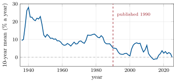
The public record agrees with the synthetic one on costs and adds a trend. Kenneth French’s short-term reversal factor (value-weighted, low minus high prior-month return, big and small stocks averaged, rebalanced monthly) earned 10.9% a year from 1926 to 1989 with a Sharpe ratio of 0.93 ( $t = 7.42$ ), and 1.6% a year from 1990 to July 2026 with a Sharpe ratio of 0.13 ( $t = 0.79$ ), before any trading costs; in the 2020s to date it has lost 5.2% a year (Figure 2.3). This is a monthly reversal on large, value-weighted portfolios, not the daily residual version, and it is not evidence that the daily effect is gone; Nagel’s results say that its returns concentrate in crises. But the long decline of the classic factor, whatever its causes (publication, cheaper trading and more capital competing to provide liquidity are the usual candidates, and these data cannot separate them), is the backdrop for every reversal book. The edge that remains belongs to whoever trades it most cheaply.

**Figure 2.3.** Kenneth French’s short-term reversal factor: the trailing 120-month mean return, annualised, at each December; the dashed line marks Jegadeesh’s and Lehmann’s papers. Derived from the Kenneth R. French Data Library (monthly ST_Rev, 202607 CRSP file); the raw series is not redistributed.

2.6 Strategy files

Strategy file 2.1 — Daily residual reversal

Who pays you, and why. Traders who need to sell or buy now, and move prices to do it; the book is paid for absorbing their flow and waiting a day.

Instruments and venues. Liquid single stocks, long and short, on their primary exchanges; the trades cross at the close or through the next session.

Signal. Minus the day’s residual return on a factor risk model, scaled by the stock’s specific volatility; skip names with earnings or other scheduled news that day.

Sizing and execution. A forecast by Grinold’s rule, a cost-aware optimiser neutral to the model’s factors, trades worked into the close.

Costs. The whole strategy: turnover of tens of per cent a day; half spread and impact on every trade; borrow on the shorts.

How it dies. Costs rise or the book grows past its capacity; news days leak into the signal; other liquidity providers compete the edge away.

Horizon, capacity, infrastructure. One to a few days; small capacity (for the chapter’s signal, below $1 billion); a daily risk model, a cost model fitted on the firm’s fills, a closing-auction execution system.

Backtest honestly. Point-in-time residuals and universe; a cost model fitted on real fills, charged on every trade; the earnings filter known in advance; results by size.

Sources. Blitz, Huij, Lansdorp and Verbeek (2013); Da, Liu and Schaumburg (2014); this chapter’s simulation.

Strategy file 2.2 — Intraday reversal to the close

Who pays you, and why. Traders who push prices during the session with temporary imbalances; the book provides the other side and unwinds as the imbalance clears.

Instruments and venues. Liquid stocks and their lit and dark venues during the session.

Signal. Minus the stock’s return over the last minutes to an hour, relative to its industry or the market, with volume and imbalance conditions.

Sizing and execution. Passive orders where possible; positions closed by the end of the day.

Costs. Spread and adverse selection dominate; the edge is of the order of a spread.

How it dies. Faster liquidity providers take the imbalance first; the move turns out to be news; bid–ask bounce mistaken for reversal.

Horizon, capacity, infrastructure. Minutes to hours; small capacity; intraday data, an order-book simulator (Book 7, chapter 18) and low-latency execution.

Backtest honestly. Trade prices, not midquotes, in the signal, and midquotes in the evaluation; a queue-aware fill model.

Sources. Heston, Korajczyk and Sadka (2010).

Strategy file 2.3 — Overnight reversal

Who pays you, and why. The two clienteles of the tug of war: overnight and opening demand that pushes prices, and daytime traders who push them back.

Instruments and venues. Liquid stocks; the opening and closing auctions.

Signal. Minus the overnight return, traded over the session; or minus the session’s return, traded overnight.

Sizing and execution. Enter at the open auction and leave at the close, or the reverse; neutral to the market and industries.

Costs. Two auction crossings a day; auction prices can move against large orders.

How it dies. The continuation within each part of the day works against it; the pattern changes with who trades at the open.

Horizon, capacity, infrastructure. Half a day; capacity limited by auction volume; open and close prices, auction imbalance data.

Backtest honestly. Official open and close prices, not the first and last trades; auction costs; no signal from an open you could not trade at.

Sources. Lou, Polk and Skouras (2019); Akbas, Boehmer, Jiang and Koch (2022).

Strategy file 2.4 — Reversal as a liquidity-provision overlay

Who pays you, and why. The same hurried traders, but the reversal is not traded alone: it tilts the trades a slower book makes anyway.

Instruments and venues. The firm’s existing equity books.

Signal. The reversal forecast added to the slower book’s forecast in the optimiser, so that the book buys its planned purchases on down days and sells on up days.

Sizing and execution. Through the slower book’s optimiser; the trades are the ones it would make anyway, with their timing shifted.

Costs. Almost none of its own: the overlay changes when trades are made, not how many.

How it dies. It does not die alone; it weakens when the slower book trades less.

Horizon, capacity, infrastructure. Days; capacity set by the host book’s turnover; the host book’s optimiser.

Backtest honestly. Compare the host book with and without the overlay at the same turnover and costs.

Sources. Nagel (2012), on reversal returns as the return to liquidity provision; Book 7, chapter 27.

2.7 Tutorial: seven before costs

Goal. Measure the three daily reversals, then trade residual reversal with costs inside the optimiser at three fund sizes. End state: the two tables and Figure 2.1.

Signals and ICs: s1_reversal.signals, ic for raw, industry-adjusted, residual and the truth, with and without earnings days.
The naive books: naive(kind) and naive(kind, 0.001), and breakeven.

The cost-aware book. A closed-form step per name and Newton’s method for the factor-neutrality multipliers.

    alpha, var, w0 = (np.asarray(a, float) for a in (alpha, var, w0))
    X = np.ones((len(alpha), 1)) if X is None else np.asarray(X, float)
    h = gamma * var
    s = (round_trip * np.asarray(half_spread, float) / h) if costs else np.zeros(len(alpha))
    c = (round_trip * eta * np.asarray(sigma, float) * np.sqrt(aum / np.asarray(adv, float)) / h) if costs \
        else np.zeros(len(alpha))

    def weights(mu):
        u = (alpha - X @ mu) / h - w0
        d = prox_cost(u, s, c)
        y = np.sqrt(np.abs(d))
        slope = np.where(np.abs(u) > s, 2 * y / np.maximum(2 * y + 1.5 * c, 1e-300), 0.0) / h   # -dw/d(X mu)
        return w0 + d, slope

    mu = np.zeros(X.shape[1])
    w, slope = weights(mu)
    for _ in range(100):
        g = X.T @ w
        if np.abs(g).max() < 1e-12:
            break
        H = X.T @ (X * slope[:, None]) + 1e-12 * np.eye(X.shape[1])
        step, t = np.linalg.solve(H, g), 1.0
        while t > 1e-6:
            w_new, slope_new = weights(mu + t * step)
            if np.abs(X.T @ w_new).sum() < np.abs(g).sum():
                break
            t /= 2
        mu, w, slope = mu + t * step, w_new, slope_new
    return w

Listing 2.1. The day’s cost-aware, factor-neutral book. code/firm/reversal/firm_reversal.py

Every day: forecast, optimise, charge the cost, drift the book.

    for t in range(START - 1, T - 1):
        ok = P.listed[t] & P.listed[t + 1] & np.isfinite(s[t]) & np.isfinite(spec[t])
        z = np.zeros(M)
        z[ok] = (s[t, ok] - s[t, ok].mean()) / s[t, ok].std()
        alpha = forecast(z, k, sig[t])
        var = np.where(ok, np.nan_to_num(spec[t]), 1.0)
        w = np.zeros(M)
        w[ok] = book(alpha[ok], var[ok], w0[ok], GAMMA, aum, sig[t, ok], adv[t, ok], HALF_SPREAD, ETA, costs,
                     round_trip, exposures(t + 1)[ok])
        dw = w - w0
        cost.append(trade_cost(dw, aum, sig[t], adv[t], HALF_SPREAD, ETA))
        gross.append(float(np.nansum(w * np.nan_to_num(R[t + 1]))))
        turn.append(float(np.abs(dw).sum()) / 2)
        gx.append(float(np.abs(w).sum()))
        w0 = w * (1 + np.nan_to_num(R[t + 1]))

Listing 2.2. The daily loop of the traded book. code/strategies-1/02-short-term-reversal/python/s1_reversal.py

Run traded(aum, costs, 1.0, skip_earnings) at $100 million, $1 billion and $10 billion, and fig_reversal.py.

What to change next. Smooth the forecast (Book 7, chapter 27) and see whether a slower book beats a faster one; restrict the universe to the 500 most liquid; multiply the cost in the optimiser by two, as if every trade had to be unwound, and explain why it does not help here.

2.8 Build: the reversal family

Purpose. The signals of the reversal family and a daily book that trades them only where they beat their costs.

Interface. raw(r), industry_adjusted(r, industry, listed), residual(r, X, w, listed), overnight(open_, prev_close), intraday(close, open_), forecast(z, ic, sigma), book(alpha, var, w0, gamma, aum, sigma, adv, half_spread, eta, costs, round_trip, X).

Rules. Signals from the day’s data only; forecasts in return units; the cost in the optimiser is the cost charged; neutrality to the exposures held exactly.

Acceptance tests. code/firm/reversal/tests/: the signals by hand; the residual orthogonal to the exposures; without costs, the book equals the closed-form mean–variance solution; costs shrink the trades; factor neutrality holds to $10^{-10}$ with costs.

Stretch. A full factor covariance in the optimiser (Book 7, chapter 27’s cost_aware); multi-period trading toward an aim portfolio (Book 7, chapter 26); the overnight and intraday signals on real open and close prices.

Sources and further reading

N. Jegadeesh, “Evidence of predictable behavior of security returns”, Journal of Finance 45(3), 1990.
B. N. Lehmann, “Fads, martingales, and market efficiency”, Quarterly Journal of Economics 105(1), 1990.
S. Nagel, “Evaporating liquidity”, Review of Financial Studies 25(7), 2012.
D. Blitz, J. Huij, S. Lansdorp and M. Verbeek, “Short-term residual reversal”, Journal of Financial Markets 16(3), 2013.
Z. Da, Q. Liu and E. Schaumburg, “A closer look at the short-term return reversal”, Management Science 60(3), 2014.
S. L. Heston, R. A. Korajczyk and R. Sadka, “Intraday patterns in the cross-section of stock returns”, Journal of Finance 65(4), 2010.
D. Lou, C. Polk and S. Skouras, “A tug of war: overnight versus intraday expected returns”, Journal of Financial Economics 134(1), 2019.
F. Akbas, E. Boehmer, C. Jiang and P. D. Koch, “Overnight returns, daytime reversals, and future stock returns”, Journal of Financial Economics 145(3), 2022.
Kenneth R. French Data Library, Short-Term Reversal Factor (ST Rev), monthly.

2.9 Exercises

Exercise 2.1 ★

The residual naive book returns 30.3% a year before costs and turns over 76% of its gross a day. Compute its break-even cost per unit traded.

Solution

Solution of Exercise 2.1.

The weight traded is twice the turnover, so the break-even cost is $0.303/(2 \times 0.76 \times 252) = 7.9$ basis points per unit traded. At ten basis points the cost is about $2 \times 0.75 \times 0.001 \times 252 = 37.8\%$ a year, more than the gross return.

Exercise 2.2 ★

A stock’s midquote does not move for two days; the spread is 10 basis points. The last trade of day one is at the bid and of day two at the ask. What return does a close-to-close file record for day two, and what does a reversal signal on trade prices conclude?

Solution

Solution of Exercise 2.2.

The recorded return is the spread, $0.001 = 10$ basis points, with no change in value. A reversal signal on trade prices sees a winner and sells it; the next day’s trade at the bid would “confirm” the reversal. That is bid–ask bounce: a reversal in the data that no one can trade, which is why signals are built on midquotes or closing auction prices, and evaluated on the prices the book could actually trade at.

Exercise 2.3 ★

With square-root impact $0.7\,\sigma\sqrt{Q/V}$ , what is the impact of a $10 million trade in a stock with daily volatility 2% and $25 million of daily volume?

Solution

Solution of Exercise 2.3.

$0.7 \times 0.02 \times \sqrt{10/25} = 0.00885$ : 88.5 basis points, on top of the half spread.

Exercise 2.4 ★★

The IC is 0.04 and a stock’s daily volatility 2%. What is Grinold’s forecast for a name two standard deviations out, and how large a trade in the stock of exercise 3 can it pay for, with a half spread of 2 basis points?

Solution

Solution of Exercise 2.4.

$0.04 \times 0.02 \times 2 = 0.0016$ , 16.0 basis points for one day. A trade of a hundredth of daily volume, $0.25 million, costs $2 + 10^4 \times 0.7 \times 0.02 \times \sqrt{0.25/25} = 16.0$ basis points: that is where the forecast stops paying. The $10 million trade of exercise 3 would cost more than five times the edge.

Exercise 2.5 ★★

Why does the residual reversal book have almost twice the raw book’s Sharpe ratio when its information coefficient is only 10% higher?

Solution

Solution of Exercise 2.5.

The Sharpe ratio depends on risk as well as return. The raw book’s losers and winners share industries and styles, so the book carries factor bets that add volatility without adding return; the residual book is nearly free of them. The return rises a little (27.0% to 30.3%), the volatility falls a lot.

Exercise 2.6 ★★

Explain why a reversal book that buys stocks on the day of a bad earnings announcement loses money in a market with post-earnings drift, and why skipping announcement days is not look-ahead.

Solution

Solution of Exercise 2.6.

On an announcement day the stock’s move is mostly news, and in a market with post-earnings drift the news keeps moving the price the same way for weeks: the reversal book buys a stock that keeps falling. Announcement dates are scheduled and published in advance, and the filter uses only whether the day was an announcement day, which is known at the close, not the surprise’s future effect.

Exercise 2.7 ★★★

Coding. Run traded(3e8, True, 1.0, True). Report the net Sharpe ratio, and explain why the net Sharpe ratio is not a monotone function of fund size in Figure 2.1.

Solution

Solution of Exercise 2.7.

The net Sharpe ratio at $300 million is 0.73. Beyond $1 billion the net ratio is within noise of zero (0.09, $-0.08$ , 0.19 at $1, $3 and $10 billion): the book trades so little that its net return is a few basis points a year, and eight years of data cannot rank such small numbers. What is robust is the fall from 1.72 at $100 million to about zero at $1 billion.

Exercise 2.8 ★★★

Find the flaw. “Our residual reversal backtest has a Sharpe ratio of 13. Even if live trading halves it, a $1 billion allocation is safe.”

Solution

Solution of Exercise 2.8.

The Sharpe ratio of 13 is before costs; after ten basis points the same book’s is $-3.43$ . The loss at size is not a halving: at $1 billion even the cost-aware book earns its costs and nothing more. The right questions are the break-even cost, the book’s turnover, and the capacity curve at the firm’s fitted costs.

2.10 Problem: Seven Before Costs

Problem 2.1

Weekend problem — a strategy that lives in its costs

The chapter’s reversal signals on firm.synthmkt, and the reversal factor on real data.

Part I — The effect.

Define short-term reversal and give the liquidity-provision explanation.
What did Jegadeesh and Lehmann find?
What did Nagel show about when reversal pays?
Why should news not reverse?

Part II — The signals.

Give the ICs of raw, industry-adjusted and residual reversal, and the truth’s.
Give the naive books’ Sharpe ratios before and after ten basis points.
Why does the residual book do so much better before costs?
What did Blitz and co-authors and Da, Liu and Schaumburg find?

Part III — Trading it.

How is the forecast put in return units?
Describe the optimiser and why it separates by name.
What does the cost-blind book trade and pay?
What does the earnings filter do, and what is it worth at $1 billion?

Part IV — The verdict.

State the named result: the net Sharpe ratio of residual reversal at $100 million and $1 billion with costs inside the optimiser, against the naive book’s.
Where is the strategy’s capacity, and why so small?
What happened to French’s reversal factor after 1989?
Why is that not proof the daily effect is gone?
What do overnight and intraday decompositions add?
Which strategy file would you run with $50 million, and which with $5 billion?
What is the single most important input to a reversal backtest?
In one sentence: what is short-term reversal, as a business?

Solution

Solution of Problem 2.1.

Recent losers outperform recent winners over the next short window; a trader who needs immediacy moves the price, and whoever absorbs the flow is paid when it comes back.
Jegadeesh: significant negative first-order serial correlation in monthly returns, 2.49% a month between extreme deciles over 1934–1987. Lehmann: weekly winners and losers reverse the next week, with profits that survive spreads and plausible costs.
Reversal returns behave like the returns to liquidity provision: predictable with the VIX, with expected returns and Sharpe ratios spiking in turmoil.
News changes the value; only the part of a move that is pressure is expected to come back.
0.037, 0.038 and 0.041; the truth 0.044 (the same in the 500 most liquid, 0.039 for the industry-adjusted).
6.69, 7.24 and 12.96 before costs; $-2.62$ , $-2.46$ and $-3.43$ after ten basis points.
It is free of the industry and style exposures that add risk without return.
Residual reversal earns risk-adjusted returns twice as large as conventional reversal and survives costs in large caps after 1990; removing the part explained by cash-flow news made the risk-adjusted return four times the standard one’s.
Grinold’s rule, $\alpha = \mathrm{IC}\,\sigma z$ , with $z$ the residual scaled by its own volatility and standardised, the IC measured before the evaluation.
Expected return less a diagonal risk penalty less the half spread and square-root impact, neutral to the fifteen factors; with diagonal risk each name’s trade is a closed-form proximal step, and the neutrality multipliers come from a small Newton iteration.
186% of capital a day at a gross exposure of 2.48; 246%, 738% and 2 293% of capital a year in costs at the three sizes.
It skips names on their announcement day; at $1 billion it turns $-0.70\%$ a year into $+0.05\%$ .
Named result. Net Sharpe ratios of 1.72 at $100 million and 0.09 at $1 billion with costs inside the optimiser, against $-27.8$ and $-31.7$ for the book that ignores them.
Below $1 billion for this signal: the edge per trade is about sixteen basis points for a name two standard deviations out, and square-root impact reaches that at 1% of a name’s daily volume.
It earned 10.9% a year (Sharpe ratio 0.93) to 1989 and 1.6% (0.13) from 1990, before costs; $-5.2\%$ a year in the 2020s to date.
It is a monthly, value-weighted factor on large portfolios; the daily residual effect is a different strategy, and reversal returns concentrate in crises.
Reversal profits are earned overnight, with continuation within each part of the day; intraday reversal is about imbalances of less than an hour and bid–ask bounce.
With $50 million the daily residual book; with $5 billion the overlay on a slower book, which costs almost nothing of its own.
The cost model: the strategy’s sign after costs depends on it.
Being paid a small fee, many times a day, for trading with people in a hurry, and keeping more of it than it costs to trade.

2.11 Interview questions

Interview question 2.1 ★ researcher, trader

Why do short-term returns reverse, and who pays the reversal trader?

Solution

Solution of Interview question 2.1.

Traders who need to trade now move prices beyond value; the price comes back as the imbalance is absorbed. The reversal trader is paid by those hurried traders, as a daily-horizon market maker, and is paid most when liquidity is scarce.

Interview question 2.2 ★★ researcher

Residual versus raw reversal: what is the difference, and why does it matter?

Solution

Solution of Interview question 2.2.

Raw reversal uses the whole return; residual reversal removes what the factor model explains. Common moves are mostly news and do not reverse, and they give the raw book factor exposures that add risk; the residual book is cleaner and, on US data and here, has a much higher risk-adjusted return.

Interview question 2.3 ★★ trader

A reversal strategy has a gross Sharpe ratio of 7 and a break-even cost of 15 basis points. Would you trade it? What would you ask?

Solution

Solution of Interview question 2.3.

Not as a naive daily book: a break-even of 15 basis points is close to real costs for most names. Ask for the cost model and its fit on real fills, the turnover, the capacity curve with costs inside the optimiser, performance by liquidity bucket and around news, and its behaviour in crises.

Interview question 2.4 ★★ developer, researcher

How would you build a daily cost-aware optimiser for a thousand names that runs in seconds?

Solution

Solution of Interview question 2.4.

Use a factor or diagonal risk model so the problem separates or nearly separates by name; the linear and power costs have a closed-form proximal step; handle neutrality with a few Lagrange multipliers found by Newton’s method, or use a proximal-gradient method (FISTA) on the factor model. Warm start from yesterday’s solution.

Interview question 2.5 ★★ risk

When does a reversal book lose money fast, and what would you monitor?

Solution

Solution of Interview question 2.5.

In a crisis when the flows it absorbs are informed or persistent (forced selling that goes on for days), when news days leak into the signal, and when a crowd of similar books unwinds. Monitor losses on news days, exposure to the factors, turnover and costs against the model, and the book’s correlation with other reversal books.

Interview question 2.6 ★★★ researcher

Under square-root impact, derive the trade size at which a one-day forecast $\alpha$ just pays for its cost, for a name with volatility $\sigma$ , daily volume $V$ and half spread $h$ .

Solution

Solution of Interview question 2.6.

The cost per unit traded of a trade of $Q$ dollars is $h + \eta\sigma\sqrt{Q/V}$ . Setting it equal to $\alpha$ gives $Q^* = V\left((\alpha - h)/(\eta\sigma)\right)^2$ for $\alpha > h$ , and no trade otherwise. With $\alpha$ = 16 basis points, $h$ = 2, $\eta = 0.7$ and $\sigma$ = 2%, $Q^* = V/100$ .

Terms defined in this chapter

See all 2333 terms in the glossary