Strategies I: Equities and Futures · Strategies

28Running a Multi-Strategy Book

In the first week of August 2007 many quantitative equity funds lost at once. Khandani and Lo, rebuilding the episode from factor and transaction data, found a market-wide deleveraging: two unwinds, on 1 August and from the open of 6 August, beginning with financials, long book-to-market and short earnings momentum, the positions many funds held under different names. A firm that runs many strategies is exposed to the same thing inside its own walls. On this chapter’s synthetic firm of ten pods, five share hidden factors that crash together three times in twenty years; detecting the overlap and capping it cuts the firm’s largest drawdown from 43.5% to 35.7% at 10% volatility, and a 5% drawdown limit on each pod stops 91.6% of healthy pods within a year. The build is firm.multistrat.

28.1 Allocation across strategies

Definition 28.1 (Multi-strategy book, pod)

A multi-strategy book is a firm’s combined portfolio of several strategies run by separate teams, allocated capital or risk by a central function that nets their trades and controls their combined risk. A pod is one such team with its own capital, risk limits and P&L.

Definition 28.2 (Strategy correlation)

Strategy correlation is the correlation between the P&L streams of two strategies; measured over normal periods it can be low while the strategies share an exposure that dominates in stress, so a firm estimates it both from P&L and from the positions’ factor exposures.

The firm’s first decision is how much risk each pod gets. Book 7, chapter 26’s risk budgeting gives the default: weights inversely proportional to each pod’s trailing volatility, so that each contributes similar risk, rebalanced monthly (Listing 28.1). The synthetic firm has ten pods at 10% volatility each, with Sharpe ratios from 0.5 to 1.0. Pods 1 to 3 load 0.4 on a shared factor, pods 4 and 5 on another; the factors are as quiet as any other noise except in three ten-day crashes, each a fall of six pod volatilities. Pod 10’s edge dies after ten years.

28.2 Netting and shared risk

Measured on twenty years of daily P&L, the three pods on the first factor have an average correlation of 0.22; a pod on neither factor, $-0.004$ with the first. The correlation understates what they share. In each crash the three pods lose 2.4 to 2.6 of their annual volatilities together, 24% to 26% of capital, in ten days. The same trade under different names is invisible in correlations measured over calm years and obvious in the pods’ positions: a risk model (Book 7, chapter 24) maps each pod’s holdings to the factors, and the firm can cap the total exposure to each.

firm at 10% volatility	no overlap control	factor cap 1.0	factor cap 0.5
Sharpe ratio	1.45	1.52	1.70
largest drawdown	43.5%	42.8%	35.7%
loss in the three crashes	31.5, 31.7, 33.6%	30.1, 30.1, 32.3%	21.6, 20.7, 22.9%

The cap limits each shared factor’s total exposure to the equivalent of one (or half) equal-weight pod, scaling down the pods that carry it. Capping at half a pod cuts each crash by about a third and raises the firm’s Sharpe ratio from 1.45 to 1.70 (Figure 28.1), because the crashes were the main cost of the overlapping pods. The losses are large because a firm of ten nearly uncorrelated pods must lever them to reach 10% volatility, and leverage multiplies whatever they share.

The synthetic firm of ten pods, scaled to 10% volatility, with and without a cap on the pods’ shared factor exposures; cumulative sums of daily returns over twenty years, the shaded bands marking the three crashes of the shared factors. Data: s1_multistrat.paths. — **Figure 28.1.** The synthetic firm of ten pods, scaled to 10% volatility, with and without a cap on the pods’ shared factor exposures; cumulative sums of daily returns over twenty years, the shaded bands marking the three crashes of the shared factors. 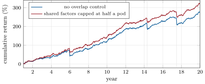Data: `s1_multistrat.paths`.

The same central view saves costs. When pods trade the same instruments, the firm executes only the net: Book 7, chapter 27’s internal crossing. Ten pods trading 200 instruments independently, each trading a fifth of them, have 34.6% of their gross volume cancel inside the firm; if all trade all, 68.5%, close to $1 - 1/\sqrt{10}$ .

28.3 Turning strategies off

Definition 28.3 (Drawdown limit)

A drawdown limit stops or cuts a strategy’s risk when its loss from its previous peak exceeds a threshold, a share of its allocated capital; it trades the cost of stopping good strategies in bad luck against the cost of running dead ones too long.

Every stop rule makes two errors. It stops pods whose edge is alive, and it lets dead ones run. Figure 28.2 shows the first: a pod with a Sharpe ratio of 0.7 at 10% volatility hits a 5% drawdown within a year on 91.6% of 20 000 simulated paths, a 10% drawdown on 34.5%, 20% on 2.1%. A limit is measured in the pod’s own volatilities: 5% is half a year’s standard deviation, well inside ordinary noise. In the synthetic firm, where stopped pods restart each year, a 5% limit stops 85.8 live pods for every hundred pod-years; at 20% it still stops 14.7, because the shared crashes push several pods through it together.

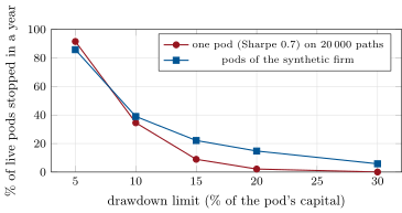
Figure 28.2. False stops: the share of pods with a live edge that hit a drawdown limit within a year, for a single pod with a Sharpe ratio of 0.7 at 10% volatility (simulated paths) and for the synthetic firm’s pods, whose shared crashes add stops. Data: s1_multistrat.limits.

The second error is the dead pod. Its Sharpe ratio falls from 0.9 to $-0.3$ after ten years; the 5% limit stops it 98 trading days later, the 10% limit after 307, the 15% limit after 979, and wider limits never, in the ten years left. A tight limit catches the dead pod quickly by catching nearly every pod quickly. The firm’s Sharpe ratio across limits (1.49 at 5%, 1.74 at 10%, 1.61 at 15%, 1.48 at 20%) peaks in the middle, and in a sample this size that peak is not a robust optimum.

28.4 Capital, drawdown limits and the pod model

The drawdown limit has a theory. Grossman and Zhou solved the problem of an investor who never wants wealth to fall below a fixed fraction of its running maximum: the optimal risky position is proportional to the distance to that floor. Risk falls as losses approach the floor instead of switching off at it, and it rises again as the surplus is rebuilt. A pod model that halves a pod’s risk at one threshold and stops it at a second is a two-step version of that rule. The central lessons of the chapter follow. Limits belong in units of each pod’s volatility and expected Sharpe ratio, not in round percentages. Shared exposures must be measured from positions, not from P&L correlations. And the firm’s capital is safest when drawdowns are controlled continuously, as Grossman and Zhou’s rule does, rather than by a cliff that stops many good pods to catch a few bad ones.

28.5 Strategy files

Strategy file 28.1 — Multi-strategy allocation with overlap control

Who pays you, and why. The pods’ combined edges, with diversification when their risks are truly different.

Instruments and venues. Whatever the pods trade.

Signal. Pods’ trailing volatility and their positions’ factor exposures.

Sizing and execution. Risk budgets by inverse volatility; caps on each shared factor; trades netted across pods.

Costs. Lower through netting; a risk model and a central execution desk.

How it dies. Crowded factors shared by many firms, as in August 2007.

Horizon, capacity, infrastructure. Continuous; position-level data from every pod.

Backtest honestly. Exposures from positions at each date; crash episodes in the sample.

Sources. Khandani and Lo (2011); this chapter: drawdown 43.5% to 35.7% with a cap of half a pod.

Strategy file 28.2 — Drawdown-controlled exposure

Who pays you, and why. Nobody: it is a risk rule that trades expected return for a floor on losses.

Instruments and venues. Any strategy or the firm.

Signal. The distance from the running peak to a floor.

Sizing and execution. Risk proportional to the surplus over the floor, or cut in steps.

Costs. False stops and the return given up after them.

How it dies. Limits set in percentages rather than volatilities; shared crashes that hit many pods together.

Horizon, capacity, infrastructure. Continuous; daily P&L.

Backtest honestly. Count false stops as well as avoided losses.

Sources. Grossman and Zhou (1993); this chapter: 91.6% of healthy pods stopped in a year at a 5% limit.

28.6 Tutorial: five at once

Goal. Run a firm of ten pods with hidden shared factors, allocate with and without overlap control, apply drawdown limits and measure false stops and the dead pod’s survival, and net trades. End state: the tables and the two figures.

Allocation and the firm: risk budgets, the factor cap, drawdown stops.

def allocate(pnl, load, t: int, window: int = 252, factor_cap: float | None = None):
    vol = pnl[max(0, t - window):t].std(0)
    w = 1 / np.maximum(vol, 1e-12)
    w /= w.sum()
    if factor_cap is not None:
        for k in range(load.shape[1]):
            expo = np.abs(load[:, k] * w * len(w)).sum()      # in units of one equal-weight pod
            if expo > factor_cap:
                on = load[:, k] != 0
                w[on] *= factor_cap / expo
        w /= w.sum()
    return w


def run_firm(S, rebalance: int = 21, factor_cap: float | None = None, limit: float | None = None):
    pnl, load = S["pnl"], S["load"]
    T, P = pnl.shape
    firm = np.zeros(T)
    alive = np.ones(P, bool)
    peak, eq = np.zeros(P), np.zeros(P)
    stops = []
    w = np.full(P, 1 / P)
    for t in range(252, T):
        if (t - 252) % rebalance == 0:
            w = allocate(pnl, load, t, 252, factor_cap)
        firm[t] = (w * alive * pnl[t]).sum()
        eq += pnl[t] * alive
        peak = np.maximum(peak, eq)
        if limit is not None:
            hit = alive & (peak - eq > limit)
            for i in np.flatnonzero(hit):
                stops.append((i, t))
            alive &= ~hit
            eq[hit] = peak[hit] = 0.0
            if (t - 252) % 252 == 0:                           # stopped pods restart at the start of each year
                alive[:] = True
    return firm, stops

Listing 28.1. Risk budgets with a factor cap, and the firm with drawdown limits. code/firm/multistrat/firm_multistrat.py

False stops and netting.

def stop_rate(sr: float, vol: float, limit: float, years: float = 1.0, n: int = 20_000, rng=None):
    rng = rng or np.random.default_rng(1)
    days = int(252 * years)
    d = vol / math.sqrt(252)
    x = np.cumsum(sr * d / math.sqrt(252) + d * rng.standard_normal((n, days)), axis=1)
    dd = np.maximum.accumulate(np.maximum(x, 0), axis=1) - x
    return float((dd.max(1) > limit).mean())


def netting(trades):
    trades = np.asarray(trades, float)
    gross = np.abs(trades).sum()
    return float(1 - np.abs(trades.sum(0)).sum() / gross)

Listing 28.2. The chance of a false stop, and netting. code/firm/multistrat/firm_multistrat.py

Run correlations(), overlap(cap), limits(limit), net_savings() and fig_multistrat.py.

What to change next. Replace the cliff with Grossman and Zhou’s proportional rule; estimate the shared factors from P&L alone and see how late they are found; plug in the P&L of this book’s own strategies (chapters 2, 5, 19 and 20) as pods.

28.7 Build: the multi-strategy firm

Purpose. Simulated pods with shared factors, risk-budget allocation with overlap control, drawdown limits, false-stop rates and netting.

Interface. PodConfig(…), simulate_pods(cfg, rng), allocate(pnl, load, t, window, factor_cap), run_firm(S, rebalance, factor_cap, limit), stop_rate(sr, vol, limit, years, n, rng), netting(trades).

Rules. Allocations from past data; loadings from positions; stopped pods restart yearly.

Acceptance tests. code/firm/multistrat/tests/: shared factors correlate pods and crash them together, the cap lowers loaded pods’ weights, netting by hand, false stops falling with the limit.

Stretch. Proportional drawdown control; capital reallocation after stops; the book’s own strategies as pods.

Sources and further reading

A. E. Khandani and A. W. Lo, “What happened to the quants in August 2007? Evidence from factors and transactions data”, Journal of Financial Markets 14(1), 2011.
S. J. Grossman and Z. Zhou, “Optimal investment strategies for controlling drawdowns”, Mathematical Finance 3(3), 1993.
L. H. Pedersen, Efficiently Inefficient: How Smart Money Invests and Market Prices Are Determined, Princeton University Press, 2015.

28.8 Exercises

Exercise 28.1 ★

Ten pods trade the same instruments with independent trades of equal size. What share of their gross volume does netting save?

Solution

Solution of Exercise 28.1.

The net of ten independent equal trades has a standard deviation $\sqrt{10}$ times one, against a gross of ten: netting saves $1 - 1/\sqrt{10} = 68.4\%$ (the simulation measures 68.5%).

Exercise 28.2 ★

A pod loads 0.4 on a factor that falls six pod volatilities in a crash. What does the pod lose, in volatilities and in percent at 10% volatility?

Solution

Solution of Exercise 28.2.

$0.4 \times 6 = 2.4$ volatilities, 24% of capital at 10% volatility.

Exercise 28.3 ★

Why do three pods with a correlation of 0.22 lose together in a crash?

Solution

Solution of Exercise 28.3.

Their correlation is measured mostly over calm days, when the shared factor is small noise; in a crash the shared factor dominates and all three move with it. A low average correlation hides a large common exposure in the tail.

Exercise 28.4 ★★

A 5% drawdown limit stops 91.6% of pods at 10% volatility within a year. What share does it stop for pods run at 5% volatility, and why?

Solution

Solution of Exercise 28.4.

34.5%: at 5% volatility a 5% limit is one annual volatility, the same as a 10% limit at 10% volatility. What matters is the limit in the pod’s own volatilities.

Exercise 28.5 ★★

Why does a tight limit catch the dead pod fastest, and at what cost?

Solution

Solution of Exercise 28.5.

Any pod, dead or alive, hits a tight limit soon; the dead pod’s negative drift makes it sooner (98 days at 5%). The cost is stopping nearly every live pod each year (91.6% on the paths), losing their edge until they restart.

Exercise 28.6 ★★

Explain Grossman and Zhou’s rule and how a two-step pod limit approximates it.

Solution

Solution of Exercise 28.6.

With wealth kept above a fraction of its running maximum, the optimal risky position is proportional to the surplus above that floor: risk shrinks smoothly as losses approach the floor and grows as the surplus is rebuilt. Halving risk at one drawdown and stopping at a second is a two-step approximation of that line.

Exercise 28.7 ★★★

Coding. Run overlap(0.25) with a stricter cap. What happens to the crashes and the Sharpe ratio, and what would you worry about in a real firm?

Solution

Solution of Exercise 28.7.

With a cap of a quarter of a pod, the crash losses fall to 12.2%, 11.1% and 13.0%, the largest drawdown to 28.0% and the Sharpe ratio rises to 1.72. In a real firm the factor map is estimated, not known: a strict cap on factors measured with error would cut pods for exposures they do not have, and would push pods toward exposures the risk model does not see.

Exercise 28.8 ★★★

Find the flaw. “Our ten pods have an average pairwise correlation of 0.05 over three years, so the firm’s risk is diversified.”

Solution

Solution of Exercise 28.8.

Three years of mostly calm data measure the correlation of noise, not of the exposures that matter in stress; the synthetic firm’s overlapping pods had 0.22 on average and lost a quarter of their capital together. Measure exposures from positions and test the firm in stress scenarios.

28.9 Problem: Five at Once

Problem 28.1

Weekend problem — a firm of pods

The chapter’s synthetic firm and the public record.

Part I — The firm.

Define a multi-strategy book, a pod and strategy correlation.
Describe the synthetic firm: pods, shared factors, crashes and the dead pod.
How does the firm allocate risk?
What did Khandani and Lo find about August 2007?

Part II — Shared risk.

Give the correlations measured over twenty years and the pods’ crash losses.
How does the firm detect the overlap?
Give the firm’s Sharpe ratio, largest drawdown and crash losses with and without the cap.
How much does netting save?

Part III — Stops.

Define a drawdown limit and its two errors.
Give the false-stop rates on simulated paths and in the firm.
How long does the dead pod run under each limit?
Why is the firm’s best limit not a robust optimum?

Part IV — The verdict.

State the named result: the firm’s drawdown with and without overlap detection, and the false-stop rate of a 5 per cent drawdown limit.
What did Grossman and Zhou show?
In what units should limits be set?
Why do shared crashes raise false stops at wide limits?
What data must every pod report to the centre?
How does this chapter relate to Book 7, chapter 28?
Which pods would you cut first after a crash, and why not all?
In one sentence: what does the centre of a multi-strategy firm add?

Solution

Solution of Problem 28.1.

A firm’s combined portfolio of strategies run by teams; one team with its own capital and limits; the correlation of their P&L, which can hide shared exposures.
Ten pods at 10% volatility, Sharpe ratios 0.5 to 1.0; pods 1–3 and 4–5 on two shared factors with three crashes; pod 10 dead after ten years.
By inverse trailing volatility, monthly.
A market-wide deleveraging in quantitative equity strategies, with unwinds on 1 and 6 August.
0.22 among pods on the same factor, $-0.004$ with others; 2.4 to 2.6 volatilities lost together in each crash.
From positions mapped to risk-model factors, capping each factor’s total exposure.
1.45, 43.5% and 31.5–33.6% without; 1.70, 35.7% and 20.7–22.9% with a cap of half a pod.
34.6% when pods trade a fifth of the instruments, 68.5% when all trade all.
A stop on a loss from the peak; stopping live pods and running dead ones.
91.6%, 34.5%, 8.9%, 2.1% and 0.0% on paths; 85.8%, 38.9%, 22.1%, 14.7% and 5.8% in the firm, for 5% to 30%.
98, 307 and 979 days at 5%, 10% and 15%; never at 20% and 30%.
One sample, five candidates, and differences within the noise.
Named result. At 10% firm volatility the largest drawdown is 43.5% without overlap detection and 35.7% with the shared factors capped at half a pod; a 5% drawdown limit stops 91.6% of healthy pods (Sharpe ratio 0.7, 10% volatility) within a year.
The optimal risky position is proportional to the surplus over a floor set as a fraction of the running maximum.
In the pod’s own volatilities and expected Sharpe ratio.
Several pods lose together, each through its own limit.
Positions and their factor exposures, daily P&L, and trades for netting.
Book 7 measured crowding across firms; this chapter measures it inside one.
The pods most exposed to the factor that crashed, reduced to the cap; the others did not cause the loss.
A view of shared risk across pods, netting, and limits set in each pod’s own units.

28.10 Interview questions

Interview question 28.1 ★ risk

How would you set a drawdown limit for a new pod?

Solution

Solution of Interview question 28.1.

From the pod’s expected volatility and Sharpe ratio: choose the limit so that the chance of stopping a pod with the expected edge within a year is acceptable (a few percent), with a soft step that halves risk first; revise as the pod’s record grows.

Interview question 28.2 ★★ risk

Two pods in different asset classes lost 8% each in the same week. What do you look for?

Solution

Solution of Interview question 28.2.

A shared exposure: map both books’ positions to common factors (crowded styles, liquidity, a common counterparty or funding source), check whether both hold the same names or trades under different labels, and look at other firms’ known positioning.

Interview question 28.3 ★★ researcher

How would you estimate whether a strategy’s edge has died, and how long would it take?

Solution

Solution of Interview question 28.3.

Compare recent performance with the distribution implied by the expected Sharpe ratio, look for a mechanism that would have killed it (crowding, costs, regime), and accept that a Sharpe ratio drop from 0.9 to $-0.3$ takes about a year or more to detect with confidence.

Interview question 28.4 ★★ developer

Design the netting of trades across pods trading the same instruments.

Solution

Solution of Interview question 28.4.

Collect pods’ orders by instrument over a short window, cross opposite orders internally at a fair reference price, send only the net to the market, and allocate fills and costs back to each pod fairly; keep an audit trail.

Interview question 28.5 ★★ trader

Your pod is 4% below its peak and the limit is 5%. What do you do, and what should the firm want you to do?

Solution

Solution of Interview question 28.5.

Reduce risk before the limit does it for you, keeping the positions with the best edge; the firm should want risk cut smoothly as the drawdown grows, not a pod that gambles to recover or one that dumps everything at the line.

Interview question 28.6 ★★★ researcher

A pod’s cumulative P&L is a Brownian motion with drift $\mu$ and volatility $\sigma$ . Using the fact that for $\mu = 0$ the drawdown from the running maximum at time $T$ is distributed as $|W_T|$ , give the probability that the drawdown exceeds $L$ at a given time $T$ , and explain why the probability that it ever exceeds $L$ within $T$ is larger.

Solution

Solution of Interview question 28.6.

For $\mu = 0$ , $P(D_T > L) = P(|W_T| > L) = 2\big(1 - \Phi(L/(\sigma\sqrt{T}))\big)$ ; for $L = 0.5\sigma$ and $T = 1$ year it is 0.617. The drawdown can exceed $L$ at some time before $T$ and recover by $T$ , so the probability that it ever exceeds $L$ within $T$ is larger; that is what a stop rule triggers on.

Terms defined in this chapter

See all 2333 terms in the glossary