Strategies I: Equities and Futures · Strategies
7Earnings
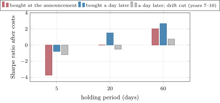
A firm reports earnings well above what the market expected, its stock jumps, and then, for weeks, it keeps drifting in the same direction. The post-earnings-announcement drift is one of the oldest anomalies in accounting research and one of the most studied; it is also one whose public record has moved against it. Chordia and co-authors found it concentrated in the most illiquid stocks, where trading costs took 70 to 100% of its paper profits, and Martineau found it non-existent in large US stocks since 2006. The synthetic market plants a clean version: 1.2% of drift per standard deviation of surprise, spread over sixty days. Traded from the day after the announcement and held for sixty days, it gives a Sharpe ratio of 2.66 after costs; held for five, ; and when the drift loses 70% of its size, as it did in the synthetic market of Book 7, chapter 13, the sixty-day book’s Sharpe ratio over the last four years falls from 3.24 to 0.75. This chapter is about trading around earnings. The build is firm.earnstrat.
7.1 Post-earnings-announcement drift
Definition 7.1 (Event study, event window)
An event study measures the average abnormal return of securities in event time, relative to the date of an event of a given kind, over an event window of days before and after it, to separate the event’s effect from the market’s.
Definition 7.2 (Post-earnings-announcement drift)
Post-earnings-announcement drift is the tendency of a stock’s abnormal returns to continue in the direction of its earnings surprise for weeks after the announcement.
Ball and Brown (1968) and Bernard and Thomas (1989) are the classic studies; Chan, Jegadeesh and Lakonishok found that past earnings surprises and past returns each predict large drifts in future returns after controlling for the other, and that analysts’ forecasts also respond sluggishly to news: a market that absorbs information gradually. The synthetic market (Book 7, chapter 5) plants exactly that: on each announcement a standard normal surprise, a jump of three daily specific volatilities per unit of surprise, and a drift of 1.2% per unit over the next sixty days. Firms announce four times a year (1.59% of stock-days are announcement days). Figure 7.1 is the chapter’s event study: for surprises above one standard deviation, the market-adjusted return is 6.94% on the announcement day and 7.75% after sixty days; below minus one, and .
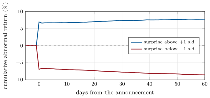
s1_earnings.car.The event study also shows the day after: the positive group gives back 0.33 points, from 6.94% to 6.61%. That is the planted one-day reversal of chapter 2 acting on the announcement’s jump, and it decides the first implementation choice below.
7.2 Analyst revisions
Definition 7.3 (Earnings-revision strategy)
An earnings-revision strategy buys stocks whose analysts have recently raised their earnings forecasts and sells stocks whose forecasts have been cut, on the evidence that forecasts, and prices with them, adjust to news gradually.
The same sluggishness that produces the drift shows in forecasts: Chan, Jegadeesh and Lakonishok found analysts’ forecasts responding slowly to past news, especially for the worst performers. A revision signal is the change in the consensus forecast over a month, scaled by price or by the dispersion of forecasts (Book 7, chapter 11). It needs a point-in-time history of individual analysts’ forecasts, which is a commercial data set; the synthetic market has no analysts, so the chapter’s strategy file on revisions rests on the published record.
7.3 Guidance and pre-announcements
Earnings news does not only arrive on the scheduled date. Firms guide their future earnings, update the guidance between reports, and sometimes pre-announce a result that will miss or beat expectations, usually in the weeks before the quarter’s report. Each of these is an event with its own window, and the drift question applies to each: does the price move fully on the day, or keep going? The engineering is the same as for announcements (a calendar of events known point in time and an event-time book), and the data problem is harder: guidance is published in press releases and on calls, not in a standardised filing, and its timestamp has to be the moment it became public. The strategy file on pre-announcements states that no performance record was verified for this book.
7.4 The announcement-day options angle
Savor and Wilson found that firms scheduled to report earned an annualised abnormal return of 9.9%, and explained it as a risk premium: announcements tell investors about other firms and the market too, so the covariance between a firm’s news and the market’s spikes around them. The synthetic market plants no announcement premium, and the portfolio of each day’s announcers, bought the close before, earns 1.8 basis points a day over the market with a statistic of 0.59: nothing.
What the synthetic market does have is the announcement’s jump: the absolute market-adjusted return on an announcement day is 3.02 times that of an ordinary day. An option expiring just after an announcement has to price that extra move, so its implied volatility should be higher than that of an option expiring just before, and should fall once the announcement is out. A straddle bought before the announcement is a bet that the move will exceed what the options priced, and a straddle sold is the opposite bet. Neither is a free lunch: both are trades on the size of the jump relative to its price (Book 9, chapter 4, trades realised against implied volatility around events).
7.5 Implementation around event dates
| drift book, synthetic market, years 3 to 10 | 5 days | 20 days | 60 days |
|---|---|---|---|
| bought at the announcement’s close: Sharpe ratio after costs | 0.02 | 2.03 | |
| bought a day later: Sharpe ratio before, after costs | 1.38, | 2.64, 1.51 | 3.31, 2.66 |
| bought a day later: net return a year; turnover a year | ; 65.2 | 4.6%; 17.2 | 5.5%; 6.6 |
| on the announcement-day return instead of the surprise | 0.85 | 2.03 | |
| drift cut by 70% from year 7: Sharpe ratio in years 7–10 | 0.75 |
Three choices decide the result. When to enter: buying at the announcement’s close means holding through the next day’s reversal of the jump, which turns the five-day book’s gross Sharpe ratio negative; waiting a day costs a day of drift and avoids it. How long to hold: the drift accrues slowly (1.2% per unit of surprise over sixty days, about two basis points a day), so a short holding period pays a full round trip for a few days of it; the five-day book trades 65 times its gross a year and its costs, 13% a year, exceed its gross return. What to measure: the reported surprise beats the announcement-day return as a signal (2.66 against 2.03 at sixty days), because the return mixes the surprise with the day’s specific noise; real books combine both, and add revisions.
And the drift can shrink. On the synthetic market whose drift loses 70% of its size from year 7 (MarketConfig.pead_break), the sixty-day book earns 4.8% a year before the break and 1.4% after, and its Sharpe ratio falls from 2.18 to 0.75; the twenty-day book goes from 1.48 to . The public record points the same way: Chordia and co-authors’ 0.04% a month in the most liquid stocks, and Martineau’s drift that vanished from large stocks after 2006.
s1_earnings.run.7.6 Strategy files
Strategy file 7.1 — SUE drift
Who pays you, and why. Investors who underreact to earnings news and adjust over weeks.
Instruments and venues. Stocks, long positive and short negative surprises.
Signal. Standardised unexpected earnings (Book 7, chapter 11) or the surprise against consensus, known at the announcement.
Sizing and execution. Event-time book, entered the day after, held up to sixty days.
Costs. The strategy’s weak point: the drift lives in illiquid stocks where costs are highest.
How it dies. Faster price discovery on the announcement day; costs; crowding.
Horizon, capacity, infrastructure. Weeks; small capacity in the stocks where the drift remains; an announcement calendar and surprise data.
Backtest honestly. Announcement timestamps (before or after the market); consensus as it stood; costs by liquidity.
Sources. Chan, Jegadeesh and Lakonishok (1996); Chordia et al. (2009): 0.04% a month in the most liquid stocks, 2.43% in the most illiquid, costs 70–100% of paper profits; Martineau (2022): none in large stocks since 2006.
Strategy file 7.2 — Revision momentum
Who pays you, and why. As for the drift: analysts and prices adjust gradually.
Instruments and venues. Stocks with analyst coverage.
Signal. The one-month change in consensus forecasts, scaled by price or dispersion.
Sizing and execution. Monthly sorts, or a signal in a multi-factor book.
Costs. Moderate turnover.
How it dies. As for the drift; herding in forecasts.
Horizon, capacity, infrastructure. Months; a point-in-time forecast history.
Backtest honestly. Forecasts dated when issued, not when entered into the database; stale forecasts removed.
Sources. Chan, Jegadeesh and Lakonishok (1996) on sluggish forecasts; no performance figure verified for this book.
Strategy file 7.4 — Straddle before announcements
Who pays you, and why. Whoever sold the options too cheaply, if the move is larger than priced; the buyer pays otherwise.
Instruments and venues. Listed equity options expiring just after the announcement.
Signal. The announcement move implied by the options against a forecast of the actual move.
Sizing and execution. Delta-hedged straddles bought or sold before, closed after.
Costs. Option spreads, wide around events.
How it dies. Implied moves that price the event correctly on average.
Horizon, capacity, infrastructure. Days; option data and a move model.
Backtest honestly. Option prices as quoted, bid and ask; the implied event move separated from ordinary volatility.
Sources. This chapter’s simulation only (announcement moves 3.02 times ordinary ones); no public performance record verified.
Strategy file 7.5 — Pre-announcement trading
Who pays you, and why. Underreaction to guidance updates and pre-announcements, if it exists.
Instruments and venues. Stocks.
Signal. Guidance changes and pre-announcements, from press releases, timestamped when public.
Sizing and execution. Event-time book as for the drift.
Costs. As for the drift.
How it dies. As for the drift.
Horizon, capacity, infrastructure. Weeks; a news feed parsed for guidance.
Backtest honestly. Public timestamps only; no information before release (chapter 17 on news).
Sources. No performance record verified for this book.
7.7 Tutorial: sixty days of drift
Goal. Trade the planted drift in event time, choose the entry day and the holding period, and watch the drift shrink. End state: the table and Figure 7.2.
The event book: names with a large recent surprise, from a delay after the announcement, for a holding window.
def _recent(x, hold, delay):
    """True at t where x had an event in [t - delay - hold + 1, t - delay]."""
    c = np.concatenate([np.zeros((1, x.shape[1])), np.cumsum(x, axis=0)])
    hi = np.maximum(np.arange(1, len(x) + 1) - delay, 0)
    lo = np.maximum(hi - hold, 0)
    return (c[hi] - c[lo]) > 0


def event_book(flag, surprise, listed, hold: int, threshold: float = 1.0, delay: int = 0):
    s = np.where(flag, np.asarray(surprise, float), 0.0)
    up = _recent((s > threshold).astype(float), hold, delay)
    down = _recent((s < -threshold).astype(float), hold, delay)
    up, down = up & listed, down & listed
    nu, nd = up.sum(axis=1, keepdims=True), down.sum(axis=1, keepdims=True)
    return np.where(up, 0.5 / np.maximum(nu, 1), 0.0) - np.where(down, 0.5 / np.maximum(nd, 1), 0.0)
Listing 7.1. The event-time book. code/firm/earnstrat/firm_earnstrat.py The event study: cumulative abnormal returns in event time.
def event_car(abret, flag, surprise, before: int, after: int, threshold: float = 0.0):
    ab = np.nan_to_num(np.asarray(abret, float))
    T = ab.shape[0]
    out = {}
    for name, sel in (("positive", surprise > threshold), ("negative", surprise < -threshold)):
        paths = []
        for t, i in zip(*np.nonzero(flag & sel), strict=True):
            if t - before >= 0 and t + after < T:
                paths.append(np.cumsum(ab[t - before:t + after + 1, i]))
        out[name] = np.mean(paths, axis=0) if paths else np.zeros(before + after + 1)
    return out
Listing 7.2. Event-time cumulative abnormal returns. code/firm/earnstrat/firm_earnstrat.py - Run
s1_earnings.run(hold, signal, cut, delay)for 5, 20 and 60 days,car,moves,announcersandfig_earnings.py.
What to change next. Weight positions by the size of the surprise; combine the surprise and the announcement return; restrict the book to the 500 most liquid names and measure what the drift is worth there.
7.8 Build: earnings strategies
Purpose. Event calendars, event-time books and event studies for earnings and other dated events.
Interface. calendar(events, T, N), event_book(flag, surprise, listed, hold, threshold, delay), announcement_move(ret, flag), event_car(abret, flag, surprise, before, after, threshold).
Rules. Events dated when public; positions from the close after the signal; holding windows fixed in advance.
Acceptance tests. code/firm/earnstrat/tests/: the calendar and the book by hand, with and without a delay; the move ratio and the event path on a planted example.
Stretch. SUE from point-in-time EPS (Book 7, chapter 11’s firm.fundpit); revision signals; the announcement calendar as a forward schedule.
Sources and further reading
- R. Ball and P. Brown, “An empirical evaluation of accounting income numbers”, Journal of Accounting Research 6(2), 1968.
- V. L. Bernard and J. K. Thomas, “Post-earnings-announcement drift: delayed price response or risk premium?”, Journal of Accounting Research 27, 1989.
- L. K. C. Chan, N. Jegadeesh and J. Lakonishok, “Momentum strategies”, Journal of Finance 51(5), 1996.
- P. Savor and M. Wilson, “Earnings announcements and systematic risk”, Journal of Finance 71(1), 2016.
- T. Chordia, A. Goyal, G. Sadka, R. Sadka and L. Shivakumar, “Liquidity and the post-earnings-announcement drift”, Financial Analysts Journal 65(4), 2009.
- C. Martineau, “Rest in peace post-earnings announcement drift”, Critical Finance Review 11(3–4), 2022.
7.9 Exercises
Exercise 7.1 ★
With a drift of 1.2% per unit of surprise over sixty days, what does a surprise of 1.5 standard deviations drift in total, and how much is that a day per unit of surprise?
Solution
Solution of Exercise 7.1.
over sixty days; per unit of surprise basis points a day.
Exercise 7.2 ★
The five-day book trades 65.2 times its gross a year and the sixty-day book 6.6 times. What does ten basis points per unit traded cost each a year?
Solution
Solution of Exercise 7.2.
The weight traded is twice the one-way turnover: a year for the five-day book, for the sixty-day book. The five-day book’s gross return, 8.3% a year, does not cover its costs.
Exercise 7.3 ★
The synthetic market reverses 5% of each day’s specific shock the next day. What does that take back from an announcement-day move of 6.94%?
Solution
Solution of Exercise 7.3.
About points, close to the 0.33 the event study shows (the move also contains market and industry parts, which are not reversed).
Exercise 7.4 ★★
Why does the reported surprise beat the announcement-day return as a signal here, and when might the return be the better one?
Solution
Solution of Exercise 7.4.
The announcement-day return is the surprise’s jump plus that day’s specific noise, so it measures the surprise with error; the reported surprise is the planted cause itself. On real data the reported surprise is measured against a consensus that may be stale or biased, and the return reflects everything announced (guidance, margins), so the return can carry information the headline number lacks. Combining both is common.
Exercise 7.5 ★★
Why is the announcement date a legitimate signal while the surprise is not known until the announcement? What must a backtest know about the timestamp?
Solution
Solution of Exercise 7.5.
The date is scheduled and published in advance; the surprise becomes public only at the announcement. A backtest must know whether each announcement came before the open, during the session or after the close, and act only from the first price after it: an after-close announcement cannot be traded at that day’s close.
Exercise 7.6 ★★
Announcement-day moves are three times ordinary ones. What does that imply for the implied volatility of an option expiring just after the announcement, compared with one expiring just before?
Solution
Solution of Exercise 7.6.
Over five trading days with one announcement day whose variance is about nine times an ordinary day’s (), the variance is ordinary days’ against 5 without the event: the implied volatility of the option spanning the announcement is about times that of one that does not, and falls back once the event is past.
Exercise 7.7 ★★★
Coding. Run run(60, ’surprise’, True). Report the Sharpe ratios before and after the break and the annual returns, and say how long you would need to watch to detect the change (Book 7, chapter 13).
Solution
Solution of Exercise 7.7.
Sharpe ratios of 2.18 before and 0.75 after the break; 4.8% a year before and 1.4% after. A drop of that size in a series with a volatility of about 2% a year takes a few years to separate from noise with Book 7, chapter 13’s break tests; waiting for certainty means trading a weakened strategy for years.
Exercise 7.8 ★★★
Find the flaw. “Our SUE backtest on all US stocks since 1990 earns 2% a month; we will run it on the S&P 500.”
Solution
Solution of Exercise 7.8.
The drift is concentrated in illiquid stocks: Chordia and co-authors found 0.04% a month in the most liquid stocks against 2.43% in the most illiquid, and Martineau none in large stocks since 2006. A backtest on all stocks says little about the S&P 500; run it on that universe, with costs, and on recent years.
7.10 Problem: Sixty Days of Drift
Problem 7.1
Weekend problem — an anomaly, traded and fading
The planted post-earnings drift of firm.synthmkt, and the public record.
Part I — The effect.
- Define an event study, an event window and the drift.
- What did Chan, Jegadeesh and Lakonishok find?
- Describe the synthetic market’s planted drift and its announcement frequency.
- Read the event study: announcement-day and sixty-day returns for both groups.
Part II — The book.
- Describe the event-time book.
- Give the Sharpe ratios at 5, 20 and 60 days, bought at the announcement and a day later.
- Why does buying at the announcement’s close hurt?
- Why do short holding periods lose after costs?
Part III — Variants.
- Surprise or announcement-day return: which wins, and why?
- What is the announcement premium, and what does the synthetic market show?
- How large are announcement moves, and what does that mean for options?
- What are revision and pre-announcement strategies, and what data do they need?
Part IV — The verdict.
- State the named result: the drift book’s Sharpe ratio at holding periods of 5, 20 and 60 days, and its fall after the planted break.
- What does the public record say about the drift in liquid and large stocks?
- Where would you still look for it?
- How would you monitor a live drift book for decay?
- What are the timestamp traps of earnings data?
- Which strategy file would you run, and at what size?
- What does the announcement premium teach about risk and anomalies?
- In one sentence: what is an earnings strategy?
Solution
Solution of Problem 7.1.
- Average abnormal returns in event time over a window around events; the drift is the continuation of abnormal returns in the surprise’s direction.
- Past surprises and past returns each predict large drifts controlling for the other; analysts’ forecasts also respond sluggishly.
- A standard normal surprise, a jump of three daily specific volatilities per unit and 1.2% of drift per unit over sixty days; four announcements a year (1.59% of stock-days).
- Above s.d.: 6.94% on the day, 7.75% at sixty days; below : and .
- Long names with a surprise above one standard deviation and short those below minus one, from a delay after the announcement for a holding window, gross one.
- At the announcement’s close: , 0.02, 2.03; a day later: , 1.51, 2.66.
- The next day reverses part of the jump (0.33 points for the positive group).
- Each position pays a full round trip for a few basis points of drift a day: costs of 13% a year at five days.
- The surprise (2.66 against 2.03 at sixty days): the return mixes the surprise with noise.
- Higher returns around scheduled announcements, 9.9% a year annualised in Savor and Wilson; none on the synthetic market (1.8 basis points a day, ).
- 3.02 times ordinary moves; options spanning the date price the jump, so their implied volatility is higher.
- Buying upward revisions of forecasts, and trading on guidance and pre-announcements; point-in-time forecast histories and timestamped press releases.
- Named result. Sharpe ratios after costs of , 1.51 and 2.66 at holding periods of 5, 20 and 60 days (bought a day after the announcement); after the drift loses 70% of its size, the sixty-day book’s Sharpe ratio over years 7–10 is 0.75 against 3.24.
- It is weak or absent in liquid stocks (0.04% a month) and absent in large stocks since 2006.
- In small, illiquid stocks, where costs eat it, and in signals the market digests more slowly (guidance, revisions, text).
- Track realised drift per unit of surprise, its event-study path, and the book’s return against a break test.
- Before-or-after-market timestamps, stale consensus, restated earnings, and announcement dates moved after the fact.
- The sixty-day drift book in the liquid names where it survives, small; or the announcement premium as a risk premium.
- That a return concentrated around events can be a reward for risk, not only a mistake.
- Positions taken around scheduled news, betting on how completely prices absorb it.
7.11 Interview questions
Interview question 7.1 ★ researcher
What is post-earnings-announcement drift, and why might it exist?
Solution
Solution of Interview question 7.1.
Abnormal returns continuing in the direction of an earnings surprise for weeks after the announcement. Explanations: investors underreact and update slowly; limits to arbitrage in the illiquid stocks where it is strongest; a risk premium the literature has not settled.
Interview question 7.2 ★★ researcher, developer
How would you build a point-in-time earnings-surprise signal? What can go wrong?
Solution
Solution of Interview question 7.2.
Actual earnings as first reported and the consensus as it stood before the announcement, both timestamped; the surprise scaled by price or by the history of surprises (SUE). What goes wrong: restated earnings replacing first reports, consensus snapshots taken after the announcement, announcement times misdated, and split-adjusted per-share numbers mixed with unadjusted ones.
Interview question 7.3 ★★ researcher
An anomaly was strong in the 1990s and is weak today. How do you decide whether to keep trading it?
Solution
Solution of Interview question 7.3.
Test for a break formally, estimate its size after the break, measure it where the book can trade (liquid names, with costs), and ask why it weakened. If the post-break return still exceeds costs with margin, keep a smaller allocation; if not, stop.
Interview question 7.4 ★★ trader
How would you trade an earnings announcement with options?
Solution
Solution of Interview question 7.4.
Compare the move implied by the options spanning the date (from the difference between their implied variance and the surrounding options’) with a forecast of the actual move; buy delta-hedged straddles when the forecast exceeds the implied move by more than costs, sell them in the opposite case.
Interview question 7.5 ★★ risk
What risks does an event-driven earnings book carry that a factor book does not?
Solution
Solution of Interview question 7.5.
Jump risk on every announcement, concentration in the names announcing that week, earnings-season clustering, and data risk (timestamps, restatements).
Interview question 7.6 ★★★ researcher
A drift of per unit of surprise accrues evenly over days; trading costs per unit traded. Find the holding period that maximises the book’s net return per unit of capital when positions enter and leave once.
Solution
Solution of Interview question 7.6.
With positions held days and replaced, there are round trips a year per unit of capital. For the net return is , increasing in ; for it is , decreasing. The optimum is to hold for the whole drift, .