Strategies I: Equities and Futures · Strategies
6Value, Quality and Low Risk
At the end of 2006 the US value factor had grown a dollar invested in 1963 to $9.77. By September 2020 it had lost 57.8% from that peak, nearly two thirds of all its gains in forty-three years, and by July 2026 it was still 29.6% below it. Over the same years the profitability factor kept earning, 2.8% a year at a Sharpe ratio of 0.51, and low-beta stocks kept earning about as much as high-beta ones. Value, quality and low risk are the canon of equity factors: the most studied, the most traded, the most argued about. This chapter builds them from point-in-time data, shows that their implementation details decide the result, and reads their record. The build is firm.factorlib.
6.1 Value: book-to-price and its cousins
Definition 6.1 (Book-to-price ratio, value strategy)
A stock’s book-to-price ratio is its book equity per share divided by its price (equivalently, book equity over market capitalisation). A value strategy buys stocks with high ratios of a fundamental measure (book equity, earnings, cash flow, sales) to price and sells stocks with low ratios.
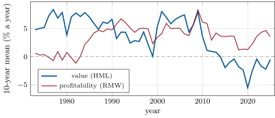
Fama and French’s 1992 study of the cross-section of expected returns is the standard reference for value, and their value factor, HML, is the average of the small and big value portfolios minus the average of the small and big growth portfolios, rebuilt each June with book equity from the previous fiscal year and market equity from the previous December. Over July 1963 to July 2026 it earned 3.6% a year at a Sharpe ratio of 0.35 (); but 5.7% a year up to 2006, over 2007–2020, and 9.4% since 2021 (Figure 6.1).
6.2 Quality and profitability
Definition 6.2 (Profitability factor, quality factor)
A profitability factor is long stocks of firms with high profitability (gross profits or operating profits over assets or book equity) and short those with low profitability. A quality factor generalises it to a composite of characteristics investors should pay more for, such as profitability, growth and safety.
Novy-Marx found that gross profits over assets predicts average returns about as well as book-to-market, that profitable firms earn more despite higher valuations, and that controlling for profitability sharply improves value strategies, especially among large stocks. Fama and French’s five-factor model (2015) adds operating profitability (RMW, robust minus weak) and investment (CMA, conservative minus aggressive). Asness, Frazzini and Pedersen defined quality as profitability, growth and safety, and found that high-quality stocks trade at higher prices but not by much, so that a quality-minus-junk factor earns significant risk-adjusted returns in the US and 24 other countries.
The appeal of the pairing is in the correlations. From 1963 to 2026, HML and RMW correlated 0.09; over value’s lost years, 2007–2020, . Value and momentum correlated , and in 2007–2020. Value and investment, on the other hand, are close relatives (0.68). Profitability kept its premium through value’s drought: 2.8% a year and a Sharpe ratio of 0.51 over 2007–2020.
On the synthetic market, which plants no profitability premium, a profitability book (four times the latest quarterly earnings over book, as filed) loses 3.8% a year at a Sharpe ratio of : it is a short-value book in disguise (its correlation with the value book is , and its signal’s IC against the planted value premium ), since a high book in the denominator makes the ratio low. A characteristic measured with the same accounting number as another factor inherits that factor’s premium with the opposite sign.
6.3 Low risk and betting against beta
Definition 6.3 (Low-risk anomaly, betting against beta)
The low-risk anomaly is the observation that low-beta and low-volatility stocks have earned higher risk-adjusted returns than high-beta and high-volatility stocks: the security market line is flatter than the capital asset pricing model predicts. Betting against beta exploits it with a portfolio long low-beta stocks levered to a beta of one and short high-beta stocks delevered to a beta of one.
Frazzini and Pedersen’s explanation is leverage aversion: investors who cannot or will not borrow buy high-beta assets to get more market exposure, bidding them up, so that high beta goes with low alpha. They found it in US equities, twenty other equity markets, Treasuries, corporate bonds and futures, and found BAB’s returns low when funding constraints tighten. French’s portfolios sorted on beta show the flat line: the lowest beta decile, with a realised beta of 0.59, earned 6.8% a year over the Treasury bill; the highest, with a beta of 1.60, earned 8.6%. The capital asset pricing model, at the market’s 7.2% excess return, says 4.3% and 11.5%. A betting-against-beta portfolio built from the extreme quintiles with rolling 60-month betas earned 4.3% a year from 1968, Sharpe ratio 0.26 (), with a beta of .
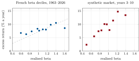
s1_fetch_value.py, s1_factors.sml.The synthetic market was built the other way: its expected returns are beta times a market premium plus the planted anomalies, and nothing rewards low beta. Its security market line is steep (the lowest trailing-beta decile earned 2.4% a year at a realised beta of 0.49, the highest 13.4% at 1.39), and a betting-against-beta book loses 5.4% a year. A strategy whose whole premise is a flat security market line has nothing to earn where the line is not flat.
6.4 Implementation details that decide the result
| synthetic value books, years 3 to 10 | Sharpe | return | beta | turnover |
|---|---|---|---|---|
| filed book, today’s price, monthly | 3.2 | |||
| filed book, today’s price, yearly | 0.21 | 1.9% | 2.5 | |
| Fama–French timing, yearly | 0.24 | 2.2% | 2.5 | |
| look-ahead book from its fiscal end, monthly | 3.2 | |||
| value and momentum composite, monthly | 0.44 | 4.0% | 0.01 | 5.1 |
The same planted value premium gives Sharpe ratios from to 0.24 depending on how book-to-price is timed. The most accurate signal (today’s price, whose rank correlation with the planted premium is 1.00) does worst, because today’s price folds in the recent return: a stock that has just fallen looks cheap, and a book rebuilt every month on today’s price is short the planted momentum (its correlation with the momentum book is ). The Fama–French convention (a book at least six months old, divided by the price of its own date) carries less of that momentum bet and does best alone. Asness and Frazzini made the same argument on real data from the other side: timely prices forecast true book-to-price better, and value portfolios built on them earned alphas of 3.05 to 3.78 percentage points a year against the standard method. On the synthetic market the combination is what pays: a composite of current-price value and momentum reaches a Sharpe ratio of 0.44, better than either. The look-ahead book, using each book value before it was filed, gains nothing here, because the synthetic book moves slowly; on real data a look-ahead of this kind is the most common way a value backtest flatters itself.
6.5 Combining the canon, and factor timing
Definition 6.4 (Factor timing)
Factor timing varies the weights of a portfolio’s factors over time according to forecasts of their returns, for instance from the spread in valuations between a factor’s long and short sides, its recent performance or its volatility.
The case for combining the canon is diversification: value, momentum and profitability each have lost decades, and their correlations are low or negative. The case for timing it is the temptation of the value spread: when cheap stocks are unusually cheap relative to expensive ones, value’s future return should be higher. Asness, Frazzini and Pedersen report the quality version of that: a low price of quality predicted a high future return of QMJ. The difficulty is that timing signals are slow, their samples short, and the record of a decade like 2007–2020, when value stayed cheap and kept losing, is the reason most practitioners hold the canon in near-fixed proportions and scale it by volatility (chapter 5) rather than time it.
6.6 Strategy files
Strategy file 6.1 — Book-to-price value
Who pays you, and why. Investors who overreact to bad news and overpay for growth, or a risk premium for distress; the literature disagrees.
Instruments and venues. Stocks, long cheap and short expensive, or long-only tilts.
Signal. Book equity over market capitalisation, point in time.
Sizing and execution. Size-neutral sorts (HML’s 2x3) or characteristic weights; rebuilt yearly or monthly.
Costs. Low turnover: two to three times the book a year here.
How it dies. Long droughts (2007–2020); growth-led markets; accounting that no longer measures value (intangibles).
Horizon, capacity, infrastructure. Years; very large capacity; point-in-time fundamentals.
Backtest honestly. Book values from their filing dates; the timing of price stated; the lost decade in the sample.
Sources. Fama and French (1992); French data: HML 3.6% a year 1963–2026, Sharpe ratio 0.35, a 57.8% drawdown from December 2006 to September 2020; Asness and Frazzini (2013).
Strategy file 6.2 — Composite value
Who pays you, and why. As for value, with the measurement error of any single ratio averaged away.
Instruments and venues. As for value.
Signal. The average z-score of several ratios to price (book, earnings, cash flow, sales), and often momentum alongside.
Sizing and execution. Sorts or characteristic weights on the composite.
Costs. As for value; more with momentum in the composite.
How it dies. As for value.
Horizon, capacity, infrastructure. Years; several fundamentals, point in time.
Backtest honestly. The composite’s ingredients fixed in advance, not chosen on the backtest.
Sources. This chapter’s simulation (value with momentum: Sharpe ratio 0.44 against 0.24 for value alone); Asness and Frazzini (2013).
Strategy file 6.3 — Gross profitability
Who pays you, and why. Investors who underprice durable profitability, or a premium the literature has not settled.
Instruments and venues. Stocks, long profitable and short unprofitable firms.
Signal. Gross profits (revenue minus cost of goods sold) over total assets.
Sizing and execution. Sorts, often combined with value.
Costs. Low turnover.
How it dies. Crowding; a denominator shared with value that turns it into a disguised value bet.
Horizon, capacity, infrastructure. Years; large capacity; income statements point in time.
Backtest honestly. Accounting data from filing dates; its correlation with the book’s other factors.
Sources. Novy-Marx (2013); French data: RMW 3.1% a year 1963–2026, Sharpe ratio 0.39.
Strategy file 6.4 — Quality minus junk
Who pays you, and why. Investors who pay too little for safe, profitable, growing firms.
Instruments and venues. Stocks in many countries.
Signal. A composite of profitability, growth and safety scores.
Sizing and execution. Long quality, short junk; neutral to size and industry.
Costs. Low turnover.
How it dies. When quality becomes expensive; the price of quality predicts its return.
Horizon, capacity, infrastructure. Years; many accounting inputs.
Backtest honestly. Every input point in time; the composite’s recipe fixed in advance.
Sources. Asness, Frazzini and Pedersen (2019): significant risk-adjusted returns in the US and 24 other countries.
Strategy file 6.5 — Betting against beta
Who pays you, and why. Leverage-constrained investors who buy high-beta assets instead of borrowing.
Instruments and venues. Stocks, bonds and futures, with leverage on the long side.
Signal. Estimated beta.
Sizing and execution. Long low beta levered to one, short high beta delevered to one.
Costs. Financing of the levered long side; shorting high-beta names.
How it dies. Tightening funding (BAB’s returns are low then); a steep security market line.
Horizon, capacity, infrastructure. Months; beta estimates, financing.
Backtest honestly. Betas known before each month; financing costs; the long side’s leverage.
Sources. Frazzini and Pedersen (2014); French beta portfolios: 4.3% a year from 1968, Sharpe ratio 0.26, before financing and trading costs.
Strategy file 6.6 — Low-volatility long-only
Who pays you, and why. As for BAB, taken as a long-only portfolio with less market risk.
Instruments and venues. Stocks, long only.
Signal. Low beta or low volatility.
Sizing and execution. The least risky quintile or a minimum-variance portfolio (Book 7, chapter 26).
Costs. Low turnover.
How it dies. Crowding into the same defensive names; rising rates hitting bond-like stocks.
Horizon, capacity, infrastructure. Years; a risk model.
Backtest honestly. Judge it on risk-adjusted return and against the market with its own beta.
Sources. French beta portfolios: the lowest decile earned 6.8% a year over bills at a beta of 0.59, 1963–2026.
6.7 Tutorial: the lost decade of value
Goal. Build value, profitability and betting-against-beta books from point-in-time fundamentals, time book-to-price four ways, and read the French record. End state: the implementation table and Figure 6.2.
Book-to-price, timed: with today’s price or with the book’s own date’s price.
def book_to_price(anchor, cum, listed, current: bool = True):
    """anchor[t, i] = log(B / P) at the anchor day plus cum[t, i] (the log price index then), NaN elsewhere. With the
    current price the signal is the latest anchor minus today's cum; held fixed it is the latest log(B / P) itself."""
    anchor, cum = np.asarray(anchor, float), np.asarray(cum, float)
    T, M = anchor.shape
    idx = np.where(np.isfinite(anchor), np.arange(T)[:, None], 0)
    idx = np.maximum.accumulate(idx, axis=0)
    last = anchor[idx, np.arange(M)[None, :]]
    base = cum[idx, np.arange(M)[None, :]]
    out = last - cum if current else last - base
    return np.where(listed & np.isfinite(last), out, np.nan)
Listing 6.1. Book-to-price from filed book values. code/firm/factorlib/firm_factorlib.py Betting against beta: each side scaled to a beta of one.
def bab_book(beta, universe, q: float = 0.2):
    b = np.where(universe, np.asarray(beta, float), np.nan)
    W = np.zeros(b.shape)
    for t in range(b.shape[0]):
        ok = np.isfinite(b[t]) & (b[t] > 0)
        n = int(ok.sum() * q)
        if n < 2:
            continue
        idx = np.flatnonzero(ok)
        order = idx[np.argsort(b[t, ok], kind="stable")]
        lo, hi = order[:n], order[-n:]
        W[t, lo] = 1.0 / n / b[t, lo].mean()
        W[t, hi] = -1.0 / n / b[t, hi].mean()
    return W
Listing 6.2. The betting-against-beta book. code/firm/factorlib/firm_factorlib.py - Run
s1_factors.run(name)for the seven books,sml(),correlations(), thens1_fetch_value.pyonce andfig_factors.py.
What to change next. Value-weight the books (the cap argument of sort_book); add the value spread as a timing signal and test it on the French sample before and after 2007; plant a profitability premium and check that the profitability book finds it.
6.8 Build: the factor library
Purpose. The equity factor canon from point-in-time characteristics, in the forms practitioners and papers use.
Interface. sort_book(signal, universe, q, cap), char_book(signal, universe), composite(*signals), bab_book(beta, universe, q), book_to_price(anchor, cum, listed, current).
Rules. Characteristics from their filing dates; the timing of prices explicit; each factor reported with its correlations to the others.
Acceptance tests. code/firm/factorlib/tests/: sort and characteristic weights by hand; composites with missing values; BAB’s zero beta; book-to-price with current and fixed prices.
Stretch. Size-neutral 2x3 sorts with NYSE breakpoints; gross profitability from income statements (Book 7, chapter 11’s firm.fundpit); value-spread timing.
Sources and further reading
- E. F. Fama and K. R. French, “The cross-section of expected stock returns”, Journal of Finance 47(2), 1992.
- R. Novy-Marx, “The other side of value: the gross profitability premium”, Journal of Financial Economics 108(1), 2013.
- C. S. Asness, A. Frazzini and L. H. Pedersen, “Quality minus junk”, Review of Accounting Studies 24(1), 2019.
- A. Frazzini and L. H. Pedersen, “Betting against beta”, Journal of Financial Economics 111(1), 2014.
- E. F. Fama and K. R. French, “A five-factor asset pricing model”, Journal of Financial Economics 116(1), 2015.
- C. Asness and A. Frazzini, “The devil in HML’s details”, Journal of Portfolio Management 39(4), 2013.
- Kenneth R. French Data Library: Fama/French 5 factors (2x3), momentum factor, portfolios formed on beta.
6.9 Exercises
Exercise 6.1 ★
HML’s cumulative wealth was $9.77 per dollar at its December 2006 peak and then fell 57.8%. What share of its cumulative gain did it lose?
Solution
Solution of Exercise 6.1.
The gain at the peak was $8.77. A 57.8% fall leaves , so the loss is $5.65 of the $8.77 gained: 64%.
Exercise 6.2 ★
A BAB book’s low-beta side has a beta of 0.6 and its high-beta side 1.5. How many dollars does it hold long and short per dollar of beta on each side, and what is its net dollar position?
Solution
Solution of Exercise 6.2.
Long of low-beta stocks and short of high-beta stocks: each side has a beta of one, and the book is net long , financed by borrowing.
Exercise 6.3 ★
The synthetic market pays 3% a year per standard deviation of book-to-price. What does a decile book earn if its long and short deciles average standard deviations, with half a dollar on each side?
Solution
Solution of Exercise 6.3.
Each side earns , so the book earns a year before costs, if the premium were the only thing its stocks carried.
Exercise 6.4 ★★
Explain why book-to-price with today’s price is negatively correlated with momentum, and why that makes value and momentum good partners.
Solution
Solution of Exercise 6.4.
Book changes slowly, so most of the month-to-month change in book-to-price is minus the stock’s return: stocks that have fallen become cheap. A current-price value book is therefore long recent losers and short recent winners, the opposite of momentum. Two strategies with positive premiums and negatively correlated returns combine into a portfolio with a higher Sharpe ratio than either.
Exercise 6.5 ★★
Why does the synthetic profitability book lose money when no profitability premium is planted?
Solution
Solution of Exercise 6.5.
Its signal, earnings over book, falls as book rises, so it ranks high-book (cheap) stocks low: the book is short value, and the synthetic market pays a value premium. Its correlation with the value book is and its signal’s IC against the planted value premium .
Exercise 6.6 ★★
At the market’s 7.2% excess return, what does the capital asset pricing model predict for betas of 0.594 and 1.604? Compare with the French deciles.
Solution
Solution of Exercise 6.6.
and . The deciles earned 6.8% and 8.6%: 2.5 points more at low beta and 2.9 points less at high beta than the model says. The security market line is flat.
Exercise 6.7 ★★★
Coding. Run run(’composite’) and correlations(). Explain the composite’s Sharpe ratio from the two books’ correlation.
Solution
Solution of Exercise 6.7.
The composite’s Sharpe ratio is 0.44. The current-price value book and the momentum book correlate , so their signals partly cancel each other’s noise: the composite keeps both premiums with less risk than either book alone.
Exercise 6.8 ★★★
Find the flaw. “Value has not worked since 2007, so it has been arbitraged away; we are dropping it.”
Solution
Solution of Exercise 6.8.
Fourteen years of losses are compatible with a premium that still exists: HML’s standard deviation is 10% a year, so a 3.6% mean has a standard error of about 2.7% over fourteen years, and value earned 9.4% a year from 2021. The drought is evidence to weigh, not proof; the better questions are whether its measurement still captures value (intangibles), and how value fits the rest of the book.
6.10 Problem: The Lost Decade of Value
Problem 6.1
Weekend problem — the canon, built and read
The French factor data and the chapter’s synthetic factor books.
Part I — Value.
- Define book-to-price and a value strategy, and describe HML’s construction.
- Give HML’s return and Sharpe ratio over the whole sample and in the three periods.
- Describe the 2007–2020 drawdown.
- Why is the timing of the price part of the definition?
Part II — Quality.
- Define the profitability and quality factors and give their published results.
- Give the correlations of HML with RMW, momentum and CMA, in the whole sample and in 2007–2020.
- What did profitability earn during value’s drought?
- Why does the synthetic profitability book lose?
Part III — Low risk.
- Define the low-risk anomaly and betting against beta.
- What does French’s beta-sorted data show, against the capital asset pricing model?
- Give the BAB portfolio’s return, Sharpe ratio and beta.
- Why does BAB lose on the synthetic market?
Part IV — The verdict.
- State the named result: the value factor’s drawdown from its 2007 peak in the French data, and the correlation of value and profitability returns.
- Rank the four timings of synthetic book-to-price and explain the ranking.
- What does combining value with momentum do here, and why?
- What did Asness and Frazzini find about timely prices?
- Define factor timing and give one argument for and one against.
- What would you check before trusting a value backtest?
- How would you allocate across the canon?
- In one sentence: what do value, quality and low risk have in common?
Solution
Solution of Problem 6.1.
- Book equity over price; buying high ratios and selling low ones. HML is half small value plus half big value minus half small growth and half big growth, rebuilt each June with the last fiscal year’s book and December’s market equity.
- 3.6% a year and 0.35 over 1963–2026; 5.7% to 2006, in 2007–2020, 9.4% since 2021.
- From $9.77 at the end of 2006 down 57.8% to September 2020; still 29.6% below the peak in July 2026.
- Book-to-price with an old price is a slow value signal; with today’s price it also loads on recent returns (short momentum).
- Long profitable, short unprofitable firms; quality adds growth and safety. Gross profitability predicts returns about as well as book-to-market; QMJ earns significant risk-adjusted returns in 25 countries.
- 0.09, and 0.68 over 1963–2026; , and 0.49 over 2007–2020.
- 2.8% a year at a Sharpe ratio of 0.51.
- It is short value in disguise, and the synthetic market pays value but not profitability.
- Low-risk stocks earn more risk-adjusted than the capital asset pricing model predicts; BAB is long levered low beta and short delevered high beta.
- The lowest decile (beta 0.59) earned 6.8% over bills and the highest (1.60) 8.6%, against 4.3% and 11.5% predicted.
- 4.3% a year from 1968, Sharpe ratio 0.26, beta .
- The synthetic market’s security market line is steep (2.4% at beta 0.49, 13.4% at 1.39): nothing rewards low beta there.
- Named result. HML fell 57.8% from its December 2006 peak to September 2020; its correlation with RMW was 0.09 over 1963–2026 and over 2007–2020.
- Fama–French timing 0.24, yearly with today’s price 0.21, look-ahead , monthly with today’s price : the more the signal folds in recent returns, the more it is short the planted momentum.
- It reaches 0.44, because current-price value and momentum correlate .
- Timely prices forecast true book-to-price better and earned alphas of 3.05–3.78 points a year against the standard method.
- Varying factor weights on forecasts of their returns. For: valuation spreads and the price of quality have predicted returns. Against: slow signals, short samples, and value’s cheapness through 2007–2020.
- Filing dates of the fundamentals, the timing of prices, the drought years in the sample, and correlations with the other factors held.
- Near-fixed weights across value, momentum and profitability, each scaled by volatility, with timing at most a small tilt.
- Each is a slow premium with long periods of losses that its partners tend to offset.
6.11 Interview questions
Interview question 6.1 ★ researcher
How is the Fama–French value factor constructed?
Solution
Solution of Interview question 6.1.
Each June, stocks are split at the NYSE median size and at the 30th and 70th NYSE percentiles of book-to-market (last fiscal year’s book over December’s market equity); HML is the average of the small and big value portfolios minus the average of the small and big growth portfolios, value-weighted, held for a year.
Interview question 6.2 ★★ researcher
Why might low-beta stocks earn higher risk-adjusted returns than high-beta stocks?
Solution
Solution of Interview question 6.2.
Investors who cannot or will not use leverage get market exposure by buying high-beta stocks, bidding them up; benchmarked managers prefer them too. High beta then comes with low alpha, and the security market line is flatter than the capital asset pricing model says.
Interview question 6.3 ★★ researcher, risk
Value lost more than half its value from 2007 to 2020. What would you conclude, and what would you not?
Solution
Solution of Interview question 6.3.
That value had a long, deep drawdown, which a 10% volatility factor can have by chance with a positive premium; that growth, low rates and intangibles dominated the period. Not that value is dead: fourteen years are not enough to tell, and it recovered part of the loss from 2021.
Interview question 6.4 ★★ researcher
Why combine value with profitability, or with momentum?
Solution
Solution of Interview question 6.4.
Their returns are uncorrelated or negatively correlated with value’s, so the combination keeps the premiums with less risk; profitability also separates cheap good firms from cheap bad ones, which improves value.
Interview question 6.5 ★★ developer, researcher
What point-in-time issues arise in building a book-to-price signal?
Solution
Solution of Interview question 6.5.
Book values known only from their filing dates, not their fiscal ends; restatements; the price used (current or at the fiscal end); share counts and splits between the book’s date and today; delisted firms kept in the history.
Interview question 6.6 ★★★ researcher
Two factors each have a Sharpe ratio of 0.3 and a correlation of . What is the Sharpe ratio of their equal-weighted combination, and of the best combination?
Solution
Solution of Interview question 6.6.
With equal weights and equal volatilities , the mean is and the variance , so the Sharpe ratio is . The best combination has , again 0.6: by symmetry equal weights are optimal.