Strategies I: Equities and Futures · Strategies
26Volatility Targeting and Risk-Managed Portfolios
When volatility jumps, every portfolio that sizes itself to a volatility target must sell, the same day, for the same reason. Moreira and Muir found that taking less risk when volatility is high raised the Sharpe ratios of the market and of most equity factors; Cederburg, O’Doherty, Wang and Yan, testing 103 strategies as a real-time investor would, found that volatility-managed portfolios do not systematically beat the unmanaged ones. On this chapter’s synthetic markets both are true: managing the market by its volatility improves the Sharpe ratio by 0.03 on average over twenty ten-year samples, and does better in only half of them. What is certain is the selling: after a synthetic 6% fall, funds holding a fifth of a percent of the market sell 14.5% of the next day’s volume. The build is firm.voltarget.
26.1 The mechanics of volatility targeting
Chapter 19 defined volatility targeting: a position sized at a target volatility divided by its forecast. A risk-managed portfolio adds a rule for the forecast and for how often to trade.
Definition 26.1 (Volatility-managed portfolio)
A volatility-managed portfolio scales an underlying portfolio’s exposure by the inverse of its forecast volatility (or variance), so that it takes less risk after volatile periods and more after calm ones, usually with a cap on leverage and a band within which the exposure is not rebalanced.
The ingredients are few (Listing 26.1): a variance forecast (the previous month’s realised variance, or an exponentially weighted one as in Book 4, chapter 18); a scaling rule, target over volatility, or Moreira and Muir’s target squared over variance, which moves exposure faster; a leverage cap; a rebalancing band. Each forecast rule and band gives a different turnover, and the turnover is the strategy’s cost.
26.2 Does it improve the Sharpe ratio?
Moreira and Muir’s argument is simple: if expected returns do not rise in proportion to volatility, scaling exposure down when volatility is high removes risk faster than it removes return. firm.synthmkt’s market factor satisfies that by construction: a constant 6% premium, GJR-GARCH volatility with a leverage effect. Twenty ten-year samples of it, held at a constant exposure or managed by the previous month’s realised variance (target 16%, leverage capped at three):
| twenty ten-year samples | constant exposure | inverse volatility | inverse variance |
|---|---|---|---|
| mean Sharpe ratio | 0.49 | 0.52 | 0.48 |
| samples better than constant | — | 10 | 8 |
| mean largest drawdown (annual volatilities) | 2.70 | 2.58 | 2.67 |
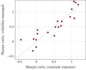
The mean gain of the inverse-volatility portfolio is 0.028, with a standard deviation of 0.22 across samples (Figure 26.1). The true Sharpe ratio of the constant portfolio is ; the samples range from to 1.18. A gain of a few hundredths is real in the model and invisible in any one decade, and the more aggressive inverse variance loses it to the noise of its own forecasts. That is Cederburg and co-authors’ finding in a laboratory: the improvement exists in the population, and a real-time investor with one history cannot count on it.
s1_voltarget.seeds.Harvey, Hoyle, Korgaonkar, Rattray, Sargaison and van Hemert found where the gain lives: only in risk assets such as equities and credit, where volatility rises when prices fall (the leverage effect); for bonds, currencies and commodities the Sharpe ratio hardly changes. What targeting does everywhere is shrink the tails, because the worst days tend to come when volatility is already high and the exposure already small. firm.synthfut’s classes have volatility clustering but no leverage effect, and targeting them at 10% changes their Sharpe ratios in both directions: 0.19 to 0.19 for equities, 0.35 to 0.28 for bonds, to for currencies, to for commodities. Their largest drawdowns fall for bonds (6.19 to 4.99 annual volatilities) and currencies (13.28 to 11.45) and rise for equities and commodities.
26.3 The industry’s footprint
Definition 26.2 (Leverage rebalancing flow)
A leverage rebalancing flow is the net trading of portfolios that follow mechanical exposure rules (volatility targets, leveraged funds’ daily resets, risk parity) in response to price and volatility changes; because many follow similar rules, the flow is concentrated and predictable from the rules and the market’s recent moves.
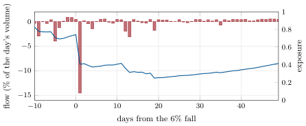
firm.voltarget’s flow simulator (Listing 26.2) puts funds holding 0.2% of a market’s value into a market that trades 0.4% of its value a day. They target 10% volatility with an exponentially weighted forecast (centre of mass 20 days, leverage capped at two). The market is calm at 12% for 250 days, falls 6% in a day, and runs at 40% for twenty days. The funds start at an exposure of 0.73; the day after the fall their forecast jumps and they sell 14.5% of the day’s volume, and over the twenty days a total of 20.5% of one day’s volume, ending at an exposure of 0.25 (Figure 26.2). All of the flow parameters are assumptions: the size of volatility-targeting money is not measured by any source fetched for this chapter.
s1_voltarget.spike.The flow moves prices, and the moves feed the forecasts. With a linear impact of 0.1 times the flow’s share of volume, the twenty days’ fall deepens from 16.6% to 18.7%; with 0.3, to 22.0%. The selling is predictable from public information (the market’s own volatility), which is what makes it a strategy file for someone else: whoever provides liquidity to deleveraging funds is paid for it.
26.4 Strategy files
Strategy file 26.1 — Volatility-managed equity
Who pays you, and why. Nobody in particular: expected returns do not rise as much as volatility, so scaling down in volatile periods improves the risk-return trade-off, if it does.
Instruments and venues. Equity index futures; equity factor portfolios.
Signal. Forecast volatility (realised or EWMA).
Sizing and execution. Exposure at target over forecast, capped; bands to limit turnover.
Costs. Turnover from forecast changes, highest with inverse variance.
How it dies. Forecast noise; instability of the relation between volatility and returns.
Horizon, capacity, infrastructure. Monthly or daily rebalancing; large capacity.
Backtest honestly. Real-time forecasts and scaling constants; compare directly with the unmanaged portfolio, not only by alpha.
Sources. Moreira and Muir (2017); Cederburg, O’Doherty, Wang and Yan (2020); this chapter: on average, better in 10 of 20 samples.
Strategy file 26.2 — Volatility-targeted multi-asset
Who pays you, and why. The asset classes’ premia, at a steadier risk.
Instruments and venues. Futures in equities, bonds, credit, commodities.
Signal. Each asset’s and the portfolio’s forecast volatility.
Sizing and execution. Scaling at asset and portfolio level; leverage cap.
Costs. Moderate.
How it dies. Correlations that jump with volatility, so that diversification disappears when the target cuts exposure.
Horizon, capacity, infrastructure. Daily to monthly; a risk system.
Backtest honestly. Forecasts from past data only; tail statistics as well as Sharpe ratios.
Sources. Harvey, Hoyle, Korgaonkar, Rattray, Sargaison and van Hemert (2018).
Strategy file 26.3 — Trading against deleveraging flow
Who pays you, and why. Volatility-targeting and other mechanical funds that must sell after volatility jumps.
Instruments and venues. Index futures near the close, when the funds rebalance.
Signal. The forecast selling: the funds’ rules applied to the market’s recent returns and an estimate of their size.
Sizing and execution. Buy into the forecast selling, exit as the pressure fades; small against the crash risk.
Costs. Low; the risk is the continuation of the fall.
How it dies. Falls that continue for fundamental reasons; competition from others who read the same flows.
Horizon, capacity, infrastructure. Days; an estimate of the funds’ assets and rules.
Backtest honestly. Only information available at the time; the crash’s continuation in the sample.
Sources. No performance figure verified; this chapter’s flow model.
26.5 Tutorial: mechanical selling
Goal. Manage the synthetic market’s volatility over twenty samples and four asset classes, and simulate the selling of targeting funds after a spike, with and without feedback. End state: the table and the two figures.
Forecasts and weights.
def realised_var(r, window: int = 21):
    r = np.asarray(r, float)
    c = np.concatenate([[0.0], np.cumsum(r**2)])
    v = np.full(len(r), np.nan)
    v[window:] = (c[window:-1] - c[:-window - 1]) / window * 252
    return v


def ewma_var(r, com: float = 20.0):
    r = np.asarray(r, float)
    lam = com / (com + 1)
    v = np.empty(len(r))
    s = np.mean(r[:21] ** 2)
    for t in range(len(r)):
        s = lam * s + (1 - lam) * r[t] ** 2
        v[t] = s * 252
    return v


def weights(var, target: float = 0.10, cap: float = 2.0, power: int = 1):
    var = np.asarray(var, float)
    w = (target / np.sqrt(var)) if power == 1 else (target**2 / var)
    return np.where(np.isnan(w), 0.0, np.minimum(w, cap))
Listing 26.1. Variance forecasts and target weights. code/firm/voltarget/firm_voltarget.py The aggregate flow: funds targeting volatility, their trade as a share of volume, and its impact fed back.
def spike_flows(base, share: float, turnover: float, impact: float, target: float = 0.10, com: float = 20.0,
                cap: float = 2.0):
    """base: the market's returns without the funds' trading. The funds hold `share` of the market's value at an
    exposure of one. On day t they trade toward target / volatility forecast at t - 1's close (capped); their net
    flow, a share of market value, divided by the daily `turnover` is a share of the day's volume, and moves that day's
    price by `impact` times that share. The forecast is updated with the realised return, impact included: the
    feedback loop."""
    base = np.asarray(base, float)
    T = len(base)
    lam = com / (com + 1)
    s = float(np.mean(base[:21] ** 2))
    w = min(cap, target / math.sqrt(s * 252))
    held = w
    r, exp_, flow = np.zeros(T), np.zeros(T), np.zeros(T)
    for t in range(T):
        new = min(cap, target / math.sqrt(s * 252))
        flow[t] = share * (new - held) / turnover
        r[t] = base[t] + impact * flow[t]
        s = lam * s + (1 - lam) * r[t] ** 2
        exp_[t] = new
        held = new * (1 + r[t])
    return {"r": r, "exposure": exp_, "flow": flow}
Listing 26.2. Targeting funds’ flow and its feedback. code/firm/voltarget/firm_voltarget.py - Run
summary(),classes()andspike(impact)for three impacts, andfig_voltarget.py.
What to change next. Add a rebalancing band and measure its effect on turnover and on the Sharpe gain; let several fund types (volatility targets, leveraged ETFs’ daily resets) trade together; let the size of the funds grow over time.
26.6 Build: volatility targeting
Purpose. Variance forecasts, target weights with caps and bands, P&L with costs, and an aggregate-flow simulator with feedback.
Interface. realised_var(r, window), ewma_var(r, com), weights(var, target, cap, power), banded(w, band), run(r, w, cost), spike_flows(base, share, turnover, impact, target, com, cap).
Rules. Forecasts from returns up to the previous close; weights capped; flows traded on the day they are decided and fed back into the forecast.
Acceptance tests. code/firm/voltarget/tests/: forecasts on a constant series, weights, the band and P&L by hand, selling after a fall and a deeper fall with feedback.
Stretch. Several fund types; bands; intraday timing of the flows.
Sources and further reading
- A. Moreira and T. Muir, “Volatility-managed portfolios”, Journal of Finance 72(4), 2017.
- S. Cederburg, M. S. O’Doherty, F. Wang and X. S. Yan, “On the performance of volatility-managed portfolios”, Journal of Financial Economics 138(1), 2020.
- C. R. Harvey, E. Hoyle, R. Korgaonkar, S. Rattray, M. Sargaison and O. van Hemert, “The impact of volatility targeting”, Journal of Portfolio Management 45(1), 2018.
26.7 Exercises
Exercise 26.1 ★
A fund targets 10% volatility. What is its exposure when the forecast is 12%? 40%?
Solution
Solution of Exercise 26.1.
and .
Exercise 26.2 ★
Funds holding 0.2% of a market’s value cut their exposure from 0.73 to 0.41 in a day; the market trades 0.4% of its value a day. What share of the day’s volume do they sell?
Solution
Solution of Exercise 26.2.
: about 16% of the day’s volume (the simulation’s 14.5% nets the day’s price drift in the funds’ exposure).
Exercise 26.3 ★
Why does inverse-variance scaling trade more than inverse-volatility scaling?
Solution
Solution of Exercise 26.3.
Exposure moves with the square of the forecast’s ratio: a forecast 10% higher cuts exposure by about 17% instead of 9%, so every forecast change is a larger trade.
Exercise 26.4 ★★
The synthetic market’s true Sharpe ratio is . What is it, what is the standard error of a ten-year estimate, and of the mean gain over twenty samples when the gains have a standard deviation of 0.22?
Solution
Solution of Exercise 26.4.
. A ten-year Sharpe ratio has a standard error of about (the samples range from to 1.18). The mean gain over twenty samples has a standard error of , so 0.028 is not significant even with twenty decades.
Exercise 26.5 ★★
Why does targeting help the Sharpe ratio of equities and not of bonds in Harvey and co-authors’ data?
Solution
Solution of Exercise 26.5.
In equities volatility rises when prices fall (the leverage effect), so volatility is high after losses and cutting exposure then avoids the worst continuation; bonds lack that link, so their volatility says little about their next returns and scaling adds only noise.
Exercise 26.6 ★★
Explain the feedback loop between targeting funds’ selling and their own volatility forecasts.
Solution
Solution of Exercise 26.6.
A volatility spike makes funds sell; their selling moves prices further; the larger moves raise the funds’ volatility forecasts; the higher forecasts make them sell more. Impact and the forecast’s memory decide how far the loop runs.
Exercise 26.7 ★★★
Coding. Run spike_flows on base_path() with a share of 0.5% and an impact of 0.3. What happens before the spike, and why?
Solution
Solution of Exercise 26.7.
Before the spike the market’s realised volatility rises from 13.0% (no impact) to 18.7%, and the funds’ exposure falls from 0.73 to 0.46: their own daily rebalancing, about 1.9% of volume on an average day, moves prices, which raises the volatility they forecast, which makes them trade more. Large enough, targeting funds generate part of the volatility they target.
Exercise 26.8 ★★★
Find the flaw. “Over 1990–2020 the volatility-managed market had an alpha of 4% against the market in a spanning regression, so we will run it.”
Solution
Solution of Exercise 26.8.
The spanning regression’s implied strategy combines the managed and unmanaged portfolios with weights estimated on the whole sample; it is not investable in real time. Compare the managed portfolio directly with the unmanaged one, out of sample, with costs, as Cederburg and co-authors did.
26.8 Problem: Mechanical Selling
Problem 26.1
Weekend problem — targeting and its footprint
The chapter’s synthetic markets and the public record.
Part I — Mechanics.
- Define a volatility-managed portfolio and a leverage rebalancing flow.
- List the ingredients of a volatility-targeting rule.
- What is Moreira and Muir’s argument?
- What did Cederburg and co-authors find?
Part II — Sharpe ratios.
- Describe the twenty-sample experiment.
- Give the mean Sharpe ratios and the number of samples improved.
- Why is a real gain invisible in one decade?
- What did Harvey and co-authors find, and what does the synthetic futures universe show?
Part III — Flows.
- Describe the flow simulation and its assumptions.
- Give the selling the day after the fall and over twenty days.
- What does feedback do to the fall?
- Why is the selling predictable?
Part IV — The verdict.
- State the named result: the Sharpe improvement from volatility management and the aggregate flow as a fraction of volume after a spike.
- What does targeting reliably do, if not raise the Sharpe ratio?
- How would you backtest a volatility-managed portfolio honestly?
- Which strategy file profits from the others?
- How does this chapter relate to chapter 19’s portfolio targeting?
- What would you need to size the deleveraging flow in a real market?
- What makes the flow dangerous to the funds themselves?
- In one sentence: what does a volatility target buy, and what does it cost the market?
Solution
Solution of Problem 26.1.
- A portfolio scaled by the inverse of forecast volatility; the net trading of funds following mechanical exposure rules.
- A variance forecast, a scaling rule, a leverage cap and a rebalancing band.
- Changes in volatility are not offset by proportional changes in expected returns, so taking less risk when volatility is high raises Sharpe ratios.
- Across 103 strategies, managed portfolios do not systematically beat unmanaged ones out of sample.
- Twenty ten-year samples of a GJR-GARCH market with a constant premium, constant or managed by last month’s realised variance.
- 0.49, 0.52 (inverse volatility) and 0.48 (inverse variance); 10 and 8 of 20 samples improved.
- The gain (0.03) is a tenth of a decade’s standard error (0.32).
- The gain holds only for risk assets with a leverage effect; the synthetic classes, without one, change in both directions.
- Funds with 0.2% of market value targeting 10%, a market trading 0.4% a day, a 6% fall and twenty days at 40% volatility; all assumed.
- 14.5% of the next day’s volume; 20.5% of a day’s volume over twenty days.
- It deepens the twenty days’ fall from 16.6% to 18.7% (impact 0.1) or 22.0% (0.3).
- It follows from the market’s own recent volatility and the funds’ public rules.
- Named result. Managing the synthetic market by its volatility raised the Sharpe ratio by 0.028 on average over twenty samples (better in 10); after a 6% fall, targeting funds holding 0.2% of the market sold 14.5% of the next day’s volume.
- It shrinks the tails and steadies the risk.
- Real-time forecasts and constants, direct comparison with the unmanaged portfolio, costs, many periods.
- Trading against deleveraging flow.
- Chapter 19 targeted a trend book’s volatility and found it levered up when the edge was small; here the question is the same for a market.
- The funds’ assets, rules and forecast windows, and the market’s volume and depth at the close.
- Their selling feeds their own forecasts.
- A steadier risk, bought with selling into falls, which the market pays for in deeper falls.
26.9 Interview questions
Interview question 26.1 ★ researcher
Why would scaling exposure by inverse volatility raise a Sharpe ratio?
Solution
Solution of Interview question 26.1.
If expected returns do not rise with volatility, a volatile period carries more risk per unit of expected return; cutting exposure then removes risk faster than return, and the ratio over time improves.
Interview question 26.2 ★★ researcher
What is wrong with judging a volatility-managed portfolio by its alpha in a spanning regression?
Solution
Solution of Interview question 26.2.
The alpha is earned by a combination of the managed and unmanaged portfolios with weights fitted on the whole sample, not available in real time; out of sample the combination’s weights are unstable and the advantage usually disappears.
Interview question 26.3 ★★ trader
Volatility doubled today. Which market participants must sell tomorrow, and how would you estimate how much?
Solution
Solution of Interview question 26.3.
Volatility-targeting funds, risk parity, leveraged ETFs resetting at the close, and option dealers short gamma; estimate each group’s assets, its rule and its forecast window, and apply today’s move to get tomorrow’s trade.
Interview question 26.4 ★★ risk
What risks does a volatility target reduce, and which does it add?
Solution
Solution of Interview question 26.4.
It reduces exposure to high-volatility periods and the severity of tail losses; it adds turnover, sells after falls, levers up in calm periods before shocks, and ties the portfolio to crowded flows.
Interview question 26.5 ★★ developer
Design the daily process that sets a volatility-targeted fund’s exposure.
Solution
Solution of Interview question 26.5.
Collect closing prices, update the forecast, compute the target exposure with caps and bands, check limits and liquidity, send orders near the close with a fallback if markets are disrupted, and log every step for reconciliation.
Interview question 26.6 ★★★ researcher
Returns are with a constant and known in advance. Show that the position has a higher Sharpe ratio than a constant position unless is constant, and compute the ratio of the two in terms of the moments of .
Solution
Solution of Interview question 26.6.
With the return is , with mean and variance . The constant position has Sharpe ratio . For small the ratio of the two is by Jensen’s inequality, with equality only when is constant.