Strategies I: Equities and Futures · Strategies
22Cross-Asset Lead–Lag
The same piece of news reaches different prices at different speeds. Hong, Torous and Valkanov found that the returns of industries such as retail, metal and petroleum forecast the whole US stock market by up to two months; Hou found that small firms follow the big firms of their own industry, most slowly after bad news; at the other end of the clock, futures and the stocks or funds that track them are linked by leads of seconds. On this chapter’s synthetic markets a lead of five days from commodities to three industries is found in two of its three links by a careful scan and traded at a Sharpe ratio of 1.73 after costs out of sample; a lead of two seconds between two assets is found in every session and pays a trader who is at most one second late. The build is firm.xasset.
22.1 Intermarket signals at daily horizons
Definition 22.1 (Intermarket signal, slow diffusion)
An intermarket signal predicts the returns of one market from the past returns of another that reflects the same fundamentals sooner, such as a commodity for its producers or a bond market for rate-sensitive stocks. Slow diffusion is the mechanism behind it: information reaches the prices of different assets at different speeds because investors specialise, attend to few markets, or face costs of trading, so prices that should move together move in sequence.
A lead–lag relationship (Book 7, chapter 10) is found by correlating one series with the other’s past. At daily horizons the candidates are many and the true links few. The chapter plants them: firm.synthmkt’s ten industry factor returns follow firm.synthfut’s ten commodities through three links, each industry receiving 0.08 times the average of one commodity’s returns over the previous five days (Listing 22.1). The effect is small: with commodity volatility of about 25% and industry volatility of 8%, each day’s lag carries a correlation of about 0.05, a t-statistic below 2 in five years.
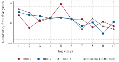
Two scans run on the first five years. The lag-by-lag scan correlates every industry with every commodity at lags of 1 to 10 days, 1 000 tests, with a Bonferroni threshold of 4.06 for a 5% family-wise error. It finds one link, the first planted one, at the right lag of five days (); the other two planted links peak at 2.7 and 3.5, below the threshold (Figure 22.1). The window scan tests one statistic per pair, the correlation of each industry with the commodity’s past five-day return, 100 tests with a threshold of 3.48. It finds the other two ( each) and misses the first (). Neither scan finds everything; neither finds anything false. A scan matched to the mechanism, here a window instead of single lags, has more power, which is why the mechanism should come before the search.
s1_xasset.daily.The links found are traded in the last five years: each linked industry is held in proportion to its commodity’s five-day return in standard deviations, capped at two, rebalanced daily at 2 basis points per unit traded. The out-of-sample Sharpe ratio is 2.09 before costs and 1.73 after, on two links. That is high because the planted diffusion is clean and constant; the public record is monthly, weaker, and changes over time.
22.2 Intraday lead–lag
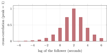
At intraday horizons the leader is usually a futures contract and the followers are the cash instruments that track it (Book 7, chapter 10’s futures-to-cash lead). The chapter simulates twenty sessions of 23 400 seconds in which a follower sees the leader’s efficient price two seconds late, both observed at random tick times (one a second on average) with noise (Listing 22.2). The Hayashi–Yoshida cross-correlation of Book 4, chapter 21 handles the asynchronous ticks without a common grid; its peak is at two seconds in every one of the twenty sessions, and its shape is symmetric about the lead (Figure 22.2).
s1_xasset.intraday.The trade: when the leader has moved more than 2 basis points over the last two seconds, buy or sell the follower in the same direction after a latency, hold two seconds, and pay half a basis point each way.
| latency (seconds) | 0 | 1 | 2 | 3 |
|---|---|---|---|---|
| trades a session | 2 343 | 2 193 | 2 025 | 1 862 |
| net return per trade (bp) | 0.73 | 0.35 | ||
| share of trades that gain | 69.6% | 57.2% | 32.0% | 25.0% |
| sessions with a positive total | 20 | 20 | 0 | 0 |
A trader who acts at once keeps most of the two-second move; one second late keeps half of it; at two seconds the follower has already moved and the trade pays the spread for nothing. The lead is the same at every latency. What changes is who can use it, as with chapter 17’s news.
22.3 Slow diffusion and who is slow
The public record says where slowness comes from. Menzly and Ozbas found that stocks in economically related supplier and customer industries predict each other’s returns, and that the cross-predictability is weaker when more informed investors follow the stocks (more analysts, more institutional ownership): specialisation makes investors slow to see news in the industries they do not cover. Hou found that the lead of big firms over small ones is mostly within industries, comes from slow adjustment to negative news, and is strongest in small, less competitive and neglected industries. Hong, Torous and Valkanov’s industries led the market by up to two months, and the industries that did so were those that also forecast economic activity. Their 2014 note, which extends the sample to 2013 with posted code, finds a robust core of leading industries but a smaller set than before, with the predictive relations changing over time. Leads decay as they become known, as most published signals do (Book 7, chapter 13).
22.4 Trading it
An intermarket strategy is built in four steps: a mechanism that says who should lead whom and at what speed; a scan matched to it, with the multiple-testing correction for the number of candidates; a test of stability in time, since leads come and go; and costs, because the predicted move is small. The daily and intraday versions differ in what limits them. At daily horizons the limit is statistical: a few true links among hundreds of candidates, each weak. At intraday horizons the limit is speed and cost: the lead is obvious, and it belongs to whoever sees it first and pays least to trade on it.
22.5 Strategy files
Strategy file 22.1 — Bond-to-equity signal
Who pays you, and why. Equity investors slow to price rate news into rate-sensitive sectors.
Instruments and venues. Bond futures as leaders; banks, utilities, real estate and other rate-sensitive stocks or sector futures as followers.
Signal. Recent bond futures returns mapped to sectors by their estimated rate sensitivity.
Sizing and execution. Sector positions sized by signal and volatility; daily.
Costs. Moderate; sector baskets or futures.
How it dies. Faster cross-asset traders; changing rate sensitivities.
Horizon, capacity, infrastructure. Days.
Backtest honestly. Sensitivities estimated from past data only; a scan corrected for every sector and lag tried.
Sources. No performance figure verified; the mechanism is slow diffusion (Hong, Torous and Valkanov, 2007).
Strategy file 22.2 — Commodity-to-producer signal
Who pays you, and why. Equity investors who specialise and follow commodity markets less closely than commodity traders.
Instruments and venues. Commodity futures as leaders; producers and heavy users as followers.
Signal. The commodity’s return over a window matched to the diffusion speed.
Sizing and execution. Long producers after commodity rises, short after falls, hedged for the market; daily or weekly.
Costs. Moderate.
How it dies. More informed investors covering both markets, as Menzly and Ozbas found.
Horizon, capacity, infrastructure. Days to weeks.
Backtest honestly. The links chosen from a mechanism, then tested; out-of-sample periods.
Sources. Hong, Torous and Valkanov (2007); Menzly and Ozbas (2010); this chapter: 1.73 after costs on two planted links.
Strategy file 22.3 — Futures-to-cash intraday lead
Who pays you, and why. Liquidity providers in the cash instruments whose quotes update after the futures’.
Instruments and venues. Index futures and the ETFs or stocks that track them.
Signal. The futures’ move over the last seconds.
Sizing and execution. Aggressive orders in the follower within the lead; small, many.
Costs. Spreads and fees on every trade; the infrastructure for speed.
How it dies. Latency competition: one second late keeps half, two seconds late loses.
Horizon, capacity, infrastructure. Seconds; co-location and direct feeds.
Backtest honestly. Timestamps as received; the follower’s quotes, not trades; queue and latency models.
Sources. No performance figure verified; this chapter’s simulation.
Strategy file 22.4 — Currency-to-exporter signal
Who pays you, and why. Equity investors slow to price currency moves into exporters’ and importers’ earnings.
Instruments and venues. Currency futures or forwards as leaders; exporters and importers as followers.
Signal. Recent currency returns times each firm’s estimated foreign revenue share.
Sizing and execution. Long exporters after the home currency weakens, short after it strengthens; hedged for the market.
Costs. Moderate.
How it dies. Firms’ hedging; faster analysts.
Horizon, capacity, infrastructure. Weeks; segment revenue data.
Backtest honestly. Revenue shares as reported at the time.
Sources. No performance figure verified.
22.6 Tutorial: same information, different speeds
Goal. Plant diffusion from commodities to industries and find it with two scans; trade what is found out of sample; simulate a two-second lead, find it with the Hayashi–Yoshida estimator and trade it at four latencies. End state: the table and the two figures.
Diffusion and the scans: planting, the lag-by-lag scan and the Bonferroni detector.
def diffuse(follow, lead, links, beta: float, lag: int):
    out = np.array(follow, float, copy=True)
    lead = np.asarray(lead, float)
    for i, j in links:
        c = np.concatenate([[0.0], np.cumsum(lead[:, i])])
        past = np.zeros(len(lead))
        t = np.arange(len(lead))
        lo = np.maximum(t - lag, 0)
        past[1:] = (c[t[1:]] - c[lo[1:]]) / lag                     # mean of lead returns t-lag .. t-1
        out[:, j] += beta * past
    return out


def lead_scan(lead, follow, lags):
    lead, follow = np.asarray(lead, float), np.asarray(follow, float)
    z = lambda x: (x - x.mean(0)) / x.std(0)  # noqa: E731
    out = np.zeros((len(lags), lead.shape[1], follow.shape[1]))
    for k, L in enumerate(lags):
        a, b = z(lead[:-L]), z(follow[L:])
        c = a.T @ b / len(a)
        out[k] = c * math.sqrt(len(a))
    return out


def detect(tstats, n_tests: int, alpha: float = 0.05):
    from statistics import NormalDist
    thr = NormalDist().inv_cdf(1 - alpha / (2 * n_tests))
    idx = np.argwhere(np.abs(tstats) > thr)
    return [tuple(int(v) for v in row) for row in idx], thr
Listing 22.1. Planted diffusion, the lagged-correlation scan and detection. code/firm/xasset/firm_xasset.py The intraday trade: act on the leader’s move after a latency.
def lead_trades(g1, g2, window: int, latency: int, hold: int, threshold: float, half_spread: float):
    """g1, g2: log prices on a 1-second grid. At each second t, if the leader moved more than `threshold` over the last
    `window` seconds, buy (or sell) the follower at t + latency and exit `hold` seconds later; one trade at a time."""
    g1, g2 = np.asarray(g1, float), np.asarray(g2, float)
    out, t = [], window
    while t + latency + hold < len(g1):
        m = g1[t] - g1[t - window]
        if abs(m) > threshold:
            a = t + latency
            out.append(np.sign(m) * (g2[a + hold] - g2[a]) - 2 * half_spread)
            t = a + hold
        else:
            t += 1
    return np.array(out)
Listing 22.2. Trading the follower after a latency. code/firm/xasset/firm_xasset.py - Run
daily()andintraday(), andfig_xasset.py.
What to change next. Let a link switch off halfway and test stability with rolling scans; correlate two leaders so that a false link appears through the correlated one; make the follower’s quotes stale only part of the time.
22.7 Build: intermarket signals
Purpose. Planted diffusion, lead scans with multiple-testing control, intermarket signals, and an intraday leader–follower simulator.
Interface. diffuse(follow, lead, links, beta, lag), lead_scan(lead, follow, lags), detect(tstats, n_tests, alpha), signal(lead, links, window, n_follow), simulate_pair(seconds, lead, vol, noise, rate, rng), lead_trades(g1, g2, window, latency, hold, threshold, half_spread).
Rules. Signals from past returns only; scans corrected for every test run; one intraday trade at a time.
Acceptance tests. code/firm/xasset/tests/: diffusion and signals by hand, a scan that finds exactly one planted lag, a lead trade by hand.
Stretch. Rolling stability tests; false discovery rate control; queue-aware intraday fills.
Sources and further reading
- H. Hong, W. Torous and R. Valkanov, “Do industries lead stock markets?”, Journal of Financial Economics 83(2), 2007; and “Note on Do Industries Lead Stock Markets”, 2014.
- L. Menzly and O. Ozbas, “Market segmentation and cross-predictability of returns”, Journal of Finance 65(4), 2010.
- K. Hou, “Industry information diffusion and the lead-lag effect in stock returns”, Review of Financial Studies 20(4), 2007.
22.8 Exercises
Exercise 22.1 ★
What two-sided z threshold gives a 5% family-wise error over 1 000 tests with Bonferroni’s correction? Over 100?
Solution
Solution of Exercise 22.1.
for 1 000 tests; for 100.
Exercise 22.2 ★
A follower receives 0.08 times the average of a leader’s last five daily returns. With volatilities of 25% for the leader and 8% for the follower, what is the correlation at one lag, and its t-statistic over 1 260 days? And for the five-day window over 1 255 days?
Solution
Solution of Exercise 22.2.
At one lag the covariance is , so the correlation is and . With the five-day window the covariance is and the window’s volatility , so the correlation is and , close to the 3.2 to 4.1 measured.
Exercise 22.3 ★
Why does the Hayashi–Yoshida estimator suit tick data that do not arrive at the same times?
Solution
Solution of Exercise 22.3.
It sums products of returns over every pair of intervals that overlap, without sampling both series on a common grid; it neither discards ticks nor creates the zero returns that previous-tick sampling does, which bias correlations toward zero (the Epps effect of Book 4).
Exercise 22.4 ★★
The trade at a latency of two seconds loses 0.51 basis points per trade after a cost of one basis point. What does it earn before costs, and why is it still positive?
Solution
Solution of Exercise 22.4.
basis points before costs. The follower’s observed price is its last tick, which arrives at random times: two seconds after the leader’s move, some of the follower’s ticks have not yet printed the move, so a little of it is still ahead in the observed prices.
Exercise 22.5 ★★
Why does the window scan find links the lag-by-lag scan misses, and the reverse?
Solution
Solution of Exercise 22.5.
The window scan adds five lags’ evidence into one statistic and pays for only 100 tests, so it has more power for a spread-out lead. The lag-by-lag scan tests each lag alone against a stricter threshold, but a lag that happens to be strong in the sample (link 1 at five days, ) can pass it while its window statistic, diluted by weaker lags, does not.
Exercise 22.6 ★★
Two commodities are strongly correlated and only one leads an industry. What can a scan report, and how would you tell?
Solution
Solution of Exercise 22.6.
It can report both: the correlated commodity inherits part of the true leader’s predictive correlation. Regress the follower on both leaders’ windows together (the false one’s coefficient should vanish), and prefer links with a mechanism.
Exercise 22.7 ★★★
Coding. Plant the diffusion at 0.12 instead of 0.08 in s1_xasset.py and rerun daily(). What does each scan find, and is every link true?
Solution
Solution of Exercise 22.7.
The lag-by-lag scan finds two links (link 3 at one day and link 1 at five), the window scan all three planted links ( of 5.3, 6.1 and 6.2) and a fourth, commodity 10 to industry 4, which is false (): it rides partly on its correlation of 0.21 with the true leader of industry 4 and partly on noise. The out-of-sample Sharpe ratio is 2.56 after costs; the false link costs a little.
Exercise 22.8 ★★★
Find the flaw. “We correlated 500 stocks with 60 futures at lags of 1 to 20 days and traded the 50 strongest pairs: backtest Sharpe ratio 3.”
Solution
Solution of Exercise 22.8.
30 000 pair-lag tests with the 50 strongest selected: most are noise, and the backtest selected them in sample. Correct for the number of tests, require a mechanism, estimate on one period and trade on another, and charge costs on 50 pairs traded daily.
22.9 Problem: Same Information, Different Speeds
Problem 22.1
Weekend problem — leads by the day and by the second
The chapter’s synthetic markets and the public record.
Part I — Diffusion.
- Define an intermarket signal and slow diffusion.
- What did Hong, Torous and Valkanov find, and what did their 2014 note add?
- What did Menzly and Ozbas find about specialisation?
- What did Hou find about big and small firms?
Part II — Daily.
- Describe the planted diffusion and its strength per lag.
- Describe the two scans and their thresholds.
- What does each scan find?
- What did the found links earn out of sample?
Part III — Intraday.
- Describe the simulated pair and the estimator used.
- Where is the cross-correlation’s peak, and how often?
- Describe the trade and its costs.
- Give the net return per trade at each latency.
Part IV — The verdict.
- State the named result: the lead detected at each horizon and the strategy’s Sharpe ratio after costs.
- What limits the daily strategy, and what limits the intraday one?
- Why should the mechanism come before the scan?
- Why do leads decay?
- How would you test a lead’s stability?
- Which strategy file needs the fastest infrastructure?
- How does this chapter relate to chapter 17?
- In one sentence: who owns a lead?
Solution
Solution of Problem 22.1.
- A prediction of one market from another’s past; information reaching prices at different speeds because investors specialise and attend to few markets.
- Industries such as retail, metal and petroleum forecast the market by up to two months; in the extended sample a robust core still does, but fewer industries, with time variation.
- Related supplier and customer industries cross-predict, less so when more informed investors follow them.
- The big-to-small lead is mostly within industries and comes from slow adjustment to bad news.
- 0.08 times the average of a commodity’s last five daily returns, in three links; about 0.05 correlation per lag.
- Lag by lag, 1 000 tests at 4.06; the five-day window, 100 tests at 3.48.
- One link at five days (); the other two links ( each), missing the first (); nothing false.
- A Sharpe ratio of 2.09 before costs and 1.73 after.
- A follower that sees the leader’s price two seconds late, both with tick noise; Hayashi–Yoshida cross-correlation.
- At two seconds, in all twenty sessions.
- Trade the follower after a leader’s move of more than 2 basis points in two seconds, hold two seconds, half a basis point each way.
- 0.73, 0.35, and basis points at latencies of 0 to 3 seconds.
- Named result. Daily: a five-day lead detected in two of three planted links by the window scan (one by the lag scan), traded at a Sharpe ratio of 1.73 after costs out of sample; intraday: a two-second lead detected in all twenty sessions, worth 0.73 basis points per trade at no latency, 0.35 at one second, and a loss from two seconds.
- Statistics (few weak links among many candidates); speed and costs.
- It sets the scan’s shape and the number of tests, which decides the power.
- Traders learn them and trade them away, as most published signals decay.
- Rolling scans, split samples, and a link switched off in simulation to see how fast the test notices.
- The futures-to-cash intraday lead.
- Chapter 17 measured how much of a news move is left at each latency; here the lead of one asset over another is the news.
- Whoever sees the leader first and trades the follower most cheaply.
22.10 Interview questions
Interview question 22.1 ★ researcher
How would you test whether one market leads another?
Solution
Solution of Interview question 22.1.
Correlate the follower’s returns with the leader’s past returns at the relevant horizons, in both directions, with an estimator suited to the data (Hayashi–Yoshida for ticks); correct for the number of lags and pairs; check stability over time and out of sample; ask for a mechanism.
Interview question 22.2 ★★ researcher
You scan 10 000 pairs and find 40 significant at 1%. What do you conclude?
Solution
Solution of Interview question 22.2.
At 1% about 100 of 10 000 would be significant by chance; 40 is fewer than chance. Nothing has been found; apply a correction for multiple tests and a mechanism before looking again.
Interview question 22.3 ★★ developer
How would you measure the lead between a futures contract and an ETF from tick data with different timestamps and clocks?
Solution
Solution of Interview question 22.3.
Synchronise clocks (use exchange timestamps, or measure and correct each feed’s delay), keep the ticks asynchronous and apply the Hayashi–Yoshida cross-correlation over a grid of lags, and read the lead from the peak or the centre of symmetry of the correlation function.
Interview question 22.4 ★★ trader
Your futures-to-cash strategy’s profit per trade halved in a month. What happened?
Solution
Solution of Interview question 22.4.
Competitors got faster, the follower’s liquidity providers started quoting off the leader, fees or spreads changed, or the firm’s own latency grew; measure the lead and the firm’s latency again.
Interview question 22.5 ★★ risk
What are the risks of an intermarket strategy that holds positions in one market based on another?
Solution
Solution of Interview question 22.5.
The link can break (a regime change, faster competitors), the follower can gap on its own news, and the position is unhedged against the follower’s specific risk; intraday, stale data or a slow feed turns the trade into adverse selection.
Interview question 22.6 ★★★ researcher
A follower’s return is with independent and . Derive the correlation of with a single lag and with the window , and the ratio of the two t-statistics.
Solution
Solution of Interview question 22.6.
, so . The window has variance and , so . With the same sample, the ratio of t-statistics is : the window has times the power of any single lag.