Strategies I: Equities and Futures · Strategies

19Trend Following

Take every liquid futures market, go long those that rose over the last year and short those that fell, and size each position so that it carries the same risk. Hurst, Ooi and Pedersen ran that rule across global markets back to 1880 and found positive average returns in every decade, low correlation with stocks and bonds, and good performance in eight of the ten worst drawdowns of a 60/40 portfolio. It is the simplest systematic strategy there is, and one of the few with a century of evidence behind it. On this chapter’s synthetic universe of forty futures the twelve-month rule earns a Sharpe ratio of 0.66 after costs over thirty years, and in the two large stock crashes the trend book gains 21% and 39% while equities lose 24% and 35%. The build is two components: firm.synthfut, the synthetic futures universe on which this and the next six chapters run, and firm.trendfollow.

Definition 19.1 (Trend following, time-series momentum)

Trend following is trading a market in the direction of its own recent price move, long after rises and short after falls, across many markets at once. Time-series momentum is its simplest rule: the position in each market has the sign of that market’s own past excess return over a lookback of $L$ days, whatever other markets did; cross-sectional momentum (chapter 5) instead ranks markets against each other.

19.1 Signal families: returns, moving averages, breakouts

Write $r_{it}$ for the daily excess return of market $i$ , the return of a position rolled in the nearby futures contract, and $P_{it} = \sum_{s \le t} r_{is}$ for its cumulative sum, a log price that ignores the roll gaps (Book 7, chapter 2’s continuous futures series). Three families of rules turn $P$ into a direction, each with a speed.

Past return. $s_{it} = \operatorname{sign}(P_{it} - P_{i,t-L})$ : time-series momentum with lookback $L$ .
Moving-average crossover. $s_{it} = \operatorname{sign}(\bar P^{(n)}_{it} - \bar P^{(m)}_{it})$ , the short average of $P$ over $n$ days against the long one over $m > n$ (Book 7, chapter 7).
Breakout. The position turns long when $P$ reaches its highest level of the last $L$ days, short at its lowest, and is kept otherwise.

Definition 19.2 (Breakout rule)

A breakout rule takes a long position when a market’s price exceeds its highest level over the last $L$ days and a short position when it falls below its lowest, and holds the position until the opposite breakout; its channel of highs and lows is also called a Donchian channel.

All three measure the same thing, the sign of a smoothed recent slope, with different weights on the past: the past return weighs the last $L$ days equally, a crossover weighs recent days more (a triangle of weights), and a breakout reacts only to new extremes, which makes it the slowest to trade. Listing 19.2 computes them, each from data up to the close of day $t$ for a position held over day $t + 1$ .

Proposition 19.3 (Trend profits are convex in the move)

Over a window of $T$ days, a position equal to the cumulative return since the window’s start, $w_t = \sum_{s < t} r_s$ , earns

\sum_{t=1}^{T} w_t r_t = \tfrac12\Big(\sum_{t=1}^{T} r_t\Big)^2 - \tfrac12 \sum_{t=1}^{T} r_t^2 .

Proof. $\big(\sum_t r_t\big)^2 = \sum_t r_t^2 + 2\sum_{s < t} r_s r_t$ , and $\sum_t w_t r_t = \sum_{s < t} r_s r_t$ . ∎

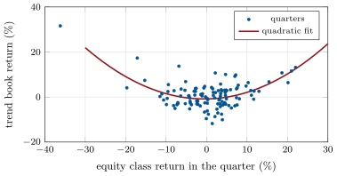
The trend follower is long the square of the window’s move and short its realised variance: it gains from large moves in either direction and loses in choppy markets where the path wanders without going anywhere. That is the shape of a long straddle, and it is why the strategy’s returns against the stock market form a smile (Figure 19.3). The sign rules are nonlinear versions of the same bet. Expected profits come from two places: the square of any persistent drift, and positive autocorrelation of returns. In the synthetic universe both come from a planted drift.

19.2 The synthetic futures universe

firm.synthfut (Listing 19.1) simulates thirty years of daily excess returns on forty markets, ten in each of four classes: equity indices, government bonds, currencies and commodities, with annual volatilities of 17.3%, 6.9%, 9.4% and 27.1% as realised. Each market has a drift that follows an AR(1) process with a half-life of a year and a standard deviation of half its volatility: the trend, planted. Each also has a carry, of which half is earned as expected return (chapter 20 trades it). Volatility clusters within each class; shocks are Student- $t$ with a factor common to the class. Three stock crashes, starting in years 7.5, 18 and 27 and lasting a hundred days each, add a steady drift of $-30\%$ to equities, $-10\%$ to commodities and $+3\%$ to bonds over the episode, make high-carry currencies fall, and raise volatility by half.

The universe is built for the whole run of futures chapters: its truth (drifts, carries, volatilities, crash dates) is kept, and curve and contracts give the log futures price for any delivery, so that chapter 21 can trade calendar spreads on its curves and chapter 23 can find its seasonal commodities.

19.3 A portfolio of trends

Each market’s position is its signal times a notional that targets 40% annual volatility divided by the number of markets, from an exponentially weighted volatility forecast with a centre of mass of sixty days (Listing 19.3); costs are 2, 1, 2 and 4 basis points per unit of notional traded for equities, bonds, currencies and commodities (assumed). The book is measured from the second year, when every signal is defined.

family	speed	Sharpe ratio after costs	before costs	turnover (times gross a year)
past return	1 month	$-0.00$	0.32	49
	3 months	0.26	0.46	29
	12 months	0.66	0.76	15
moving averages	5/20 days	0.10	0.32	33
	20/100 days	0.43	0.48	9
	50/250 days	0.72	0.76	5
breakout	20 days	0.17	0.29	18
	55 days	0.34	0.39	8
	250 days	0.78	0.80	3

Within each family the slow rule wins, because the planted drift is slow; across families at the same speed the results are close, because the rules measure the same slope. Costs separate the fast rules: the one-month rule turns its gross over 49 times a year and its Sharpe ratio of 0.32 before costs becomes nothing after them. By lookback (Figure 19.1) the Sharpe ratio rises to six months and is flat beyond: a longer lookback measures the drift with less noise but reacts later to its changes, and at a half-life of a year the two balance over a broad range. Moskowitz, Ooi and Pedersen found the same range in 58 real markets: persistence for one to twelve months, partially reversing beyond.

Time-series momentum on the synthetic universe of forty futures, thirty years: the Sharpe ratio after costs of the volatility-scaled sign-of-past-return rule by lookback. The planted drifts have a half-life of a year. Data: s1_trend.lookbacks. — **Figure 19.1.** Time-series momentum on the synthetic universe of forty futures, thirty years: the Sharpe ratio after costs of the volatility-scaled sign-of-past-return rule by lookback. The planted drifts have a half-life of a year. 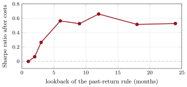Data: `s1_trend.lookbacks`.

A practitioner does not know the speed of the trends to come, so trend books blend speeds. The blend of the three past-return rules, averaging their positions, earns 0.40; the blend of all nine rules, 0.55. Both are below the best single rule, which is what hindsight costs: the best rule is known only after the fact, and choosing it among nine is the selection that Book 7, chapter 20’s overfitting measures penalise. Blending is insurance against the speed of the next trend being different from the last.

19.4 Volatility scaling

Definition 19.4 (Volatility targeting)

Volatility targeting sizes a position, or a whole portfolio, so that its forecast volatility equals a fixed target: the notional is the target divided by the forecast, recomputed as the forecast changes, usually with a cap on leverage.

Trend books use it at two levels. Per market, it makes a bond future and a natural-gas future carry the same risk, so that the book is diversified in risk and not dominated by the most volatile markets. Replacing the three past-return rules’ volatility-scaled positions with equal notional positions drops the blend’s Sharpe ratio from 0.40 to 0.31: the commodities dominate the equal-notional book and the bonds hardly count. Baltas and Kosowski show that the choice of volatility estimator matters too, mainly through turnover.

At the portfolio level, targeting 10% raises the blend’s realised volatility from 7.7% to 10.2% and lowers its Sharpe ratio from 0.40 to 0.34; the largest drawdown, 3.7 annual standard deviations untargeted, is 3.8 targeted. In this model the book’s volatility is mostly a measure of how many markets trend together: when they disagree, the book’s volatility falls and the target levers it up, just when its edge is small. Portfolio targeting is a risk decision, not an alpha, and chapter 26 measures when it helps.

19.5 The long record and crisis alpha

Definition 19.5 (Crisis alpha)

Crisis alpha is a strategy’s tendency to earn positive returns during prolonged declines of the stock market, measured as its return over the market’s largest drawdowns; for trend following it comes from being short equities and positioned for the flight to quality once the decline has lasted longer than the signal’s lookback.

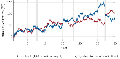
The synthetic crashes show the mechanism (Figure 19.2). The first, in year 7.5, happened to be small (equities lost 6.8% over its hundred days, the planted fall offset by the noise) and the trend book, at 10% volatility, gained 2.3%. In the second, equities fell 24.3% and the book gained 21.1%; in the third, 35.1% and 39.0%. The gains come once the declines are under way: the signals turn short equities and long bonds a few weeks in, and the steady fall does the rest. A crash that happens in a day, like 19 October 1987 (Book 6, chapter 22), gives the signals no time and earns nothing.

The blended trend book, targeted at 10% volatility, and the mean of the ten equity index futures on the synthetic universe, as cumulative sums of daily excess returns; the shaded bands are the three planted stock crashes. Data: s1_trend.paths. — **Figure 19.2.** The blended trend book, targeted at 10% volatility, and the mean of the ten equity index futures on the synthetic universe, as cumulative sums of daily excess returns; the shaded bands are the three planted stock crashes. Data: `s1_trend.paths`.

Quarter by quarter, the book’s returns against the equity class’s form the smile of the convexity proposition (Figure 19.3): a quadratic fitted to the 115 quarters has a curvature of 2.63, and the worst equity quarter ( $-36.2\%$ ) was the book’s best ( $+31.6\%$ ). Across all quarters the correlation is $-0.09$ : the trend book is not a short on stocks, but a long position in large moves.

The trend smile: the blended trend book’s quarterly return (10% volatility target) against the equity class’s, 115 quarters of the synthetic universe, with a fitted quadratic (curvature 2.63). Data: s1_trend.smile. — **Figure 19.3.** The trend smile: the blended trend book’s quarterly return (10% volatility target) against the equity class’s, 115 quarters of the synthetic universe, with a fitted quadratic (curvature 2.63). Data: `s1_trend.smile`.

The public record is longer than any synthetic one. Moskowitz, Ooi and Pedersen found a diversified time-series momentum portfolio with substantial abnormal returns, little exposure to standard factors and its best performance in extreme markets; Hurst, Ooi and Pedersen extended the evidence to 1880, with positive average returns in every decade and good performance in eight of the ten largest crisis periods.

One market can be tested on real data here: NYMEX WTI crude oil, from the EIA’s daily settlements of the first two contracts (Book 3, chapter 2), rolled five days before expiry into a continuous series. The twelve-month rule, at a 40% volatility target, earned 9.0% a year from 1986 to 2024 at a Sharpe ratio of 0.22, long on 54% of days; holding the future long earned a Sharpe ratio of 0.04. One market is a small sample (a Sharpe ratio measured over 38 years has a standard error of about 0.16), and trend following’s case rests on the many markets that diversify it.

19.6 The recent decade

A long record does not guarantee the next decade. Baltas and Kosowski study the underperformance of time-series momentum after the global financial crisis and relate it to the level of pairwise correlations between markets: when every market moves with every other, the book holds one position forty times. The synthetic universe gives the other half of the answer, sampling noise. The blended book, whose planted edge is the same throughout, had Sharpe ratios of 0.56, 0.24 and 0.34 in its three decades. A decade’s Sharpe ratio has a standard error of about $1/\sqrt{10} = 0.32$ , so a strategy with a true Sharpe ratio of 0.4 will show anything from 0.08 to 0.72 in most decades. A bad decade is weak evidence that the edge has gone; a mechanism that explains why it would have gone (correlations, crowding, costs) is stronger.

19.7 Strategy files

Strategy file 19.1 — Time-series momentum

Who pays you, and why. Hedgers who trade against trends, and investors who underreact to news and overreact later; speculators profit at hedgers’ expense in Moskowitz, Ooi and Pedersen’s data.

Instruments and venues. Liquid futures in equity indices, bonds, currencies and commodities.

Signal. The sign of each market’s past 12-month excess return.

Sizing and execution. Volatility-scaled positions, rebalanced daily or weekly; futures rolled before expiry.

Costs. Low: a turnover of about fifteen times gross a year at a twelve-month lookback.

How it dies. Correlated markets; choppy markets without persistent moves; crowding.

Horizon, capacity, infrastructure. Months; large capacity in the liquid futures; a roll and margin operation.

Backtest honestly. Rolled contracts with their costs; volatility forecasts known at the time; lookback not chosen in hindsight.

Sources. Moskowitz, Ooi and Pedersen (2012); this chapter: 0.66 after costs on the synthetic universe.

Strategy file 19.2 — Moving-average crossover portfolio

Who pays you, and why. As for time-series momentum.

Instruments and venues. As for time-series momentum.

Signal. The sign of a short minus a long moving average of each market’s price, for example 50/250 days.

Sizing and execution. Volatility-scaled; the crossover trades less often than the past-return rule at a similar speed.

Costs. Lowest of the three families at the slow speeds (five times gross a year at 50/250 here).

How it dies. As for time-series momentum.

Horizon, capacity, infrastructure. Months; as for time-series momentum.

Backtest honestly. The pair of windows fixed before the test, or chosen with Book 7’s overfitting controls.

Sources. Baltas and Kosowski (2020) on trading rules and turnover; this chapter: 0.72.

Strategy file 19.3 — Breakout system

Who pays you, and why. As for time-series momentum; breakouts also meet stop orders placed at recent highs and lows.

Instruments and venues. Liquid futures.

Signal. New $L$ -day highs and lows (20, 55 or 250 days).

Sizing and execution. Volatility-scaled; orders at the channel, often as stops.

Costs. Slippage at breakouts, when many stops trigger together.

How it dies. False breakouts in ranges; crowded stops.

Horizon, capacity, infrastructure. Weeks to months.

Backtest honestly. Fills at the breakout level plus slippage, not at the day’s close.

Sources. No performance figure verified; this chapter: 0.78 at 250 days, 0.17 at 20.

Strategy file 19.4 — Multi-speed trend blend

Who pays you, and why. As for time-series momentum, at every horizon.

Instruments and venues. Liquid futures.

Signal. The average of rules at several speeds and families.

Sizing and execution. Positions averaged before trading, so that offsetting rules net.

Costs. Those of the fast components, reduced by netting.

How it dies. As for time-series momentum.

Horizon, capacity, infrastructure. Weeks to a year.

Backtest honestly. The set of speeds fixed in advance; compare with the best single rule only as hindsight.

Sources. Hurst, Ooi and Pedersen (2017); this chapter: 0.55 for nine rules, 0.40 for three speeds of one.

Strategy file 19.5 — Volatility-scaled trend portfolio

Who pays you, and why. As for time-series momentum.

Instruments and venues. Liquid futures across the four classes.

Signal. Any trend rule.

Sizing and execution. Each market at the same forecast volatility; the portfolio optionally at a volatility target with a leverage cap.

Costs. Extra turnover from volatility changes; efficient estimators reduce it.

How it dies. Volatility forecasts that lag regime changes.

Horizon, capacity, infrastructure. As for the rule; a daily volatility pipeline.

Backtest honestly. Forecasts from past data only; leverage caps as they would have applied.

Sources. Moskowitz, Ooi and Pedersen (2012); Baltas and Kosowski (2020); this chapter: 0.40 scaled against 0.31 equal notional.

Strategy file 19.6 — Trend on WTI crude futures

Who pays you, and why. Producers and consumers hedging, and the slow adjustment of oil prices to supply shocks.

Instruments and venues. NYMEX WTI crude futures, rolled before expiry.

Signal. The sign of the past 12-month return of the rolled series.

Sizing and execution. A 40% volatility target, rolled five days before expiry.

Costs. The roll’s spread and the curve’s shape (contango costs a long position).

How it dies. As one market, it is not diversified: it dies with oil’s regime.

Horizon, capacity, infrastructure. Months.

Backtest honestly. The rolled series, not the nearby price; April 2020’s negative settlement handled by rolling early.

Sources. EIA settlements; this chapter: a Sharpe ratio of 0.22, 1986–2024.

19.8 Tutorial: crisis alpha

Goal. Build the synthetic futures universe, run the trend rules at three speeds in three families, blend and scale them, and measure the book in the planted crashes and on real crude oil. End state: the table and the three figures.

The universe: drifts, carries, volatility states, class factors and crashes, day by day.

    for t in range(T):
        a = phi_a * a + math.sqrt(1 - phi_a**2) * cfg.trend_sr * sig * rng.standard_normal(N)
        c = cmean + phi_c * (c - cmean) + math.sqrt(1 - phi_c**2) * 0.8 * csd * rng.standard_normal(N)
        lv = cfg.vol_persist * lv + math.sqrt(1 - cfg.vol_persist**2) * cfg.vol_sd * rng.standard_normal(K)
        boost = math.log(cfg.crash_vol) if in_crash[t] else 0.0
        vol_t = sig * np.exp(lv[cls] - cfg.vol_sd**2 / 2 + boost) / math.sqrt(YEAR)
        shock = np.sqrt(w) * _student(rng, cfg.t_df, K)[cls] + np.sqrt(1 - w) * _student(rng, cfg.t_df, N)
        mu = (a + cfg.carry_premium * c) / YEAR
        if in_crash[t]:
            mu = mu + np.array(cfg.crash_move)[cls] / cfg.crash_days
            fx = cls == 2
            z = (c[fx] - c[fx].mean()) / (c[fx].std() + 1e-12)
            mu[fx] -= cfg.carry_crash * z / cfg.crash_days
        out["r"][t] = mu + vol_t * shock
        out["carry"][t], out["drift"][t], out["vol"][t] = c, a, vol_t

Listing 19.1. One day of the synthetic futures universe. code/firm/synthfut/firm_synthfut.py

The signals: volatility forecast, past return, moving-average crossover and breakout.

def ewma_vol(r, com: float = 60.0):
    r = np.asarray(r, float)
    lam = com / (com + 1.0)
    v = np.empty_like(r)
    s = np.nanmean(r[:21] ** 2, axis=0)
    for t in range(len(r)):
        s = lam * s + (1 - lam) * r[t] ** 2
        v[t] = s
    return np.sqrt(252 * v)


def tsmom(r, L: int):
    c = np.cumsum(np.asarray(r, float), axis=0)
    out = np.zeros_like(c)
    out[L:] = np.sign(c[L:] - c[:-L])
    return out


def ma_cross(r, short: int, long: int):
    c = np.cumsum(np.asarray(r, float), axis=0)
    cs = np.cumsum(np.vstack([np.zeros((1, c.shape[1])), c]), axis=0)
    out = np.zeros_like(c)
    ms = (cs[long:] - cs[long - short:-short]) / short
    ml = (cs[long:] - cs[:-long]) / long
    out[long - 1:] = np.sign(ms - ml)
    return out


def breakout(r, L: int):
    c = np.cumsum(np.asarray(r, float), axis=0)
    out = np.zeros_like(c)
    state = np.zeros(c.shape[1])
    for t in range(L, len(c)):
        window = c[t - L:t]
        state = np.where(c[t] >= window.max(0), 1.0, np.where(c[t] <= window.min(0), -1.0, state))
        out[t] = state
    return out

Listing 19.2. Trend signals and the volatility forecast. code/firm/trendfollow/firm_trendfollow.py

The book: positions, P&L net of costs, and the portfolio volatility target.

def positions(signal, vol, target: float = 0.4, n: int | None = None):
    n = n or np.asarray(signal).shape[1]
    return np.asarray(signal) * target / (n * np.maximum(np.asarray(vol), 1e-4))


def run(r, pos, cost):
    """cost: per unit of notional traded, scalar or (N,)."""
    r, pos = np.asarray(r, float), np.asarray(pos, float)
    pnl = np.zeros(len(r))
    pnl[1:] = (pos[:-1] * r[1:]).sum(1)
    trade = np.abs(np.diff(pos, axis=0, prepend=np.zeros((1, pos.shape[1]))))
    pnl -= (trade * np.asarray(cost)).sum(1)
    return pnl


def vol_target(pnl, target: float = 0.10, com: float = 60.0, cap: float = 3.0):
    pnl = np.asarray(pnl, float)
    v = ewma_vol(pnl[:, None], com)[:, 0]
    lev = np.minimum(target / np.maximum(v, 1e-6), cap)
    out = np.zeros_like(pnl)
    out[1:] = lev[:-1] * pnl[1:]
    return out

Listing 19.3. Positions, P&L and volatility targeting. code/firm/trendfollow/firm_trendfollow.py

Run table(), lookbacks(), summary(), crises(), smile(), decades() and wti(), and fig_trend.py.

What to change next. Shorten the drifts’ half-life and find the best lookback; make a crash happen in five days instead of a hundred; replace the sign with a continuous signal (the past return divided by its volatility) and compare turnover.

19.9 Build: futures universe and trend library

Purpose. firm.synthfut: a deterministic futures universe with planted drifts, carry, volatility clustering, crashes and seasonal curves, for chapters 19 to 25. firm.trendfollow: trend signals, volatility-scaled positions, P&L with costs and portfolio targeting.

Interface. FutConfig(…), simulate_futures(cfg), season(amp, phase, t), curve(F, t, taus), contracts(F, t, n, every); ewma_vol, tsmom, ma_cross, breakout, positions, run, vol_target.

Rules. Signals use data up to the close of $t$ for positions held over $t + 1$ ; the universe keeps its truth; futures returns carry no seasonality (the curve anticipates it).

Acceptance tests. code/firm/synthfut/tests/ and code/firm/trendfollow/tests/: shapes and determinism, class volatilities, a crash’s fall, the curve’s slope equal to the carry; signals on a hand-made path, P&L and costs by hand, the volatility forecast and target.

Stretch. Continuous signals; an EWMA crossover family; roll schedules and contract-level P&L.

Sources and further reading

T. J. Moskowitz, Y. H. Ooi and L. H. Pedersen, “Time series momentum”, Journal of Financial Economics 104(2), 2012.
B. Hurst, Y. H. Ooi and L. H. Pedersen, “A century of evidence on trend-following investing”, Journal of Portfolio Management 44(1), 2017.
N. Baltas and R. Kosowski, “Demystifying time-series momentum strategies: volatility estimators, trading rules and pairwise correlations”, in Market Momentum, Wiley, 2020.
US Energy Information Administration, NYMEX WTI crude oil futures daily settlements, contracts 1 and 2.

19.10 Exercises

Exercise 19.1 ★

An exponentially weighted variance with a centre of mass of 60 days has a decay factor $\lambda = 60/61$ . What is it, and what is the weights’ half-life in days?

Solution

Solution of Exercise 19.1.

$\lambda = 60/61 = 0.9836$ ; the weights halve after $\ln 0.5/\ln \lambda = 42$ days.

Exercise 19.2 ★

A book of 40 markets targets 40% volatility per market divided by 40. What notional, as a share of capital, does it hold in a commodity with 25% volatility, and in a bond future with 6%?

Solution

Solution of Exercise 19.2.

$0.4/(40 \times 0.25) = 0.04$ , 4% of capital in the commodity; $0.4/(40 \times 0.06) = 0.167$ , 16.7% in the bond future. Each contributes 1% of volatility.

Exercise 19.3 ★

Use the convexity proposition to explain why a trend follower loses in a market that rises 5% and falls 5% repeatedly.

Solution

Solution of Exercise 19.3.

Over each up-and-down cycle the total move is zero, so the first term, $\tfrac12(\sum r)^2$ , is zero, and the book loses half the realised variance: it buys after the rise and sells after the fall. Choppy markets are the trend follower’s cost, as time decay is a straddle holder’s.

Exercise 19.4 ★★

The smile’s fitted quadratic is $2.63x^2 + 0.03x - 0.01$ in quarterly returns. What does it predict for the trend book in a quarter when equities fall 30%?

Solution

Solution of Exercise 19.4.

$2.63 \times 0.09 + 0.03 \times (-0.30) - 0.01 = 0.218$ : about 22% in the quarter, if the fall is gradual like the synthetic crashes.

Exercise 19.5 ★★

Why does the one-month rule, with a Sharpe ratio of 0.32 before costs, earn nothing after them, while the 250-day breakout loses almost nothing to costs?

Solution

Solution of Exercise 19.5.

The one-month rule turns its gross over 49 times a year and the 250-day breakout 3 times; at a few basis points per unit traded, costs grow with turnover while the fast rule’s gross edge is small. The breakout’s Sharpe ratio drops only from 0.80 to 0.78.

Exercise 19.6 ★★

A trend book’s true Sharpe ratio is 0.4. Roughly what range of decade Sharpe ratios should you expect, and what do you conclude from a decade at 0.1?

Solution

Solution of Exercise 19.6.

A decade’s Sharpe ratio has a standard error of about $1/\sqrt{10} = 0.32$ , so most decades fall between $0.4 - 0.32 = 0.08$ and $0.4 + 0.32 = 0.72$ . A decade at 0.1 is within that range: on its own it is weak evidence that the edge has gone. Look for a mechanism (correlations, crowding, costs) before concluding.

Exercise 19.7 ★★★

Coding. Simulate the universe with FutConfig(trend_half_life=63.0) and rerun lookbacks((3, 6, 12)). Which lookback is best, and why is it not three months?

Solution

Solution of Exercise 19.7.

Twelve months is still best (0.42), then six (0.39), then three (0.13). A three-month lookback would follow the faster drift, but it measures it with much more noise: the past return over $L$ days has a drift part growing with $L$ and a noise part growing with $\sqrt{L}$ . At this drift strength the noise dominates short lookbacks, so the best lookback stays long even though the trends are faster; all Sharpe ratios fall.

Exercise 19.8 ★★★

Find the flaw. “We tested 200 combinations of lookbacks and moving-average windows on our 40 futures and the best earned a Sharpe ratio of 1.3 after costs; we will run it.”

Solution

Solution of Exercise 19.8.

The best of 200 correlated trials is selected on noise: its expected Sharpe ratio is inflated by the maximum of many estimates, each with a standard error of about 0.2 over 25 years. Deflate it (Book 7, chapter 20), or blend the rules and judge the blend; out of sample, expect much less.

19.11 Problem: Crisis Alpha

Problem 19.1

Weekend problem — a trend book through three crashes

The chapter’s synthetic futures universe, the WTI series and the public record.

Part I — Rules.

Define trend following, time-series momentum and a breakout rule.
Write the three signal families and say how they weight the past.
State and prove the convexity proposition.
What two sources of expected profit does a trend rule have?

Part II — The universe and the book.

Describe firm.synthfut’s drifts, carries, volatility and crashes.
How are positions sized, and what do costs assume?
Give the Sharpe ratios after costs of the nine rules.
Why do slow rules win here, and what does blending cost and buy?

Part III — Scaling and crises.

Define volatility targeting; compare volatility-scaled and equal-notional books.
What does portfolio targeting do to the blend, and why?
Define crisis alpha and give the book’s returns in the three crashes.
Describe the smile and its curvature.

Part IV — The verdict.

State the named result: the trend portfolio’s return in the simulated stock crashes and its Sharpe ratio across speeds.
What did the twelve-month rule earn on WTI, and how much should one market convince you?
What did Moskowitz, Ooi and Pedersen, and Hurst, Ooi and Pedersen find?
What do Baltas and Kosowski relate the recent underperformance to?
How noisy is a decade’s Sharpe ratio?
Which crash would trend following not protect against?
How does this chapter’s momentum differ from chapter 5’s?
In one sentence: what does a trend follower own?

Solution

Solution of Problem 19.1.

Trading each market in the direction of its own recent move; the sign of the past $L$ -day return; a position at new $L$ -day highs or lows, held until the opposite.
Past return (equal weights over $L$ days); moving-average crossover (a triangle of weights, more on recent days); breakout (only new extremes).
$\sum_t w_t r_t = \tfrac12(\sum_t r_t)^2 - \tfrac12\sum_t r_t^2$ , from expanding the square.
The square of persistent drifts and positive autocorrelation of returns.
AR(1) drifts with a half-life of a year and a standard deviation of half the volatility; carries of which half is earned; volatility clustering by class; three hundred-day crashes.
Signal times 40% over 40 markets over an EWMA volatility forecast; 2, 1, 2 and 4 basis points per unit traded by class.
Past return $-0.00$ , 0.26, 0.66; crossovers 0.10, 0.43, 0.72; breakouts 0.17, 0.34, 0.78.
The planted drift is slow; blending costs the difference to the best rule (0.55 for nine rules against 0.78) and buys insurance against choosing the wrong speed.
Sizing to a forecast volatility; 0.40 scaled against 0.31 at equal notional.
It raises volatility from 7.7% to 10.2% and lowers the Sharpe ratio from 0.40 to 0.34: it levers up when markets disagree and the edge is small.
Positive returns in prolonged stock declines; $+2.3\%$ , $+21.1\%$ and $+39.0\%$ while equities lost 6.8%, 24.3% and 35.1%.
Quarterly returns against equities are U-shaped, curvature 2.63; the worst equity quarter was the book’s best.
Named result. In the three synthetic crashes the trend book at 10% volatility returned $+2.3\%$ , $+21.1\%$ and $+39.0\%$ against equity losses of 6.8%, 24.3% and 35.1%; the Sharpe ratio after costs rises with speed from $-0.00$ (one month) to 0.66 (twelve months) for past returns, 0.10 to 0.72 for crossovers and 0.17 to 0.78 for breakouts.
9.0% a year at a Sharpe ratio of 0.22, 1986–2024; with a standard error of about 0.16, not much.
Persistence for one to twelve months in 58 markets and substantial abnormal returns; positive returns in every decade since 1880 and good performance in eight of ten crises.
The level of pairwise correlations between markets.
A standard error of about 0.32.
A sudden crash, such as 19 October 1987, faster than the signals’ lookback.
Chapter 5 ranks stocks against each other and is market-neutral; here each market is traded on its own past, and the book can be net long or short.
Large moves, in either direction, paid for with losses in choppy markets.

19.12 Interview questions

Interview question 19.1 ★ researcher

What is the difference between time-series and cross-sectional momentum?

Solution

Solution of Interview question 19.1.

Time-series momentum trades each asset on its own past return and can be net long or short the whole market; cross-sectional momentum ranks assets against each other, long winners and short losers, and is neutral by construction.

Interview question 19.2 ★★ researcher

Why do trend followers scale positions by volatility?

Solution

Solution of Interview question 19.2.

So that each market contributes similar risk: without it the most volatile markets dominate and the book is not diversified; and so that the book’s risk is steadier through volatility regimes.

Interview question 19.3 ★★ researcher, trader

Your trend book has lost money for two years. How do you decide whether to keep running it?

Solution

Solution of Interview question 19.3.

Compare the loss with the distribution of two-year returns implied by the book’s expected Sharpe ratio; check whether the mechanism has changed (correlations, crowding, costs, market access); check the implementation (rolls, costs, sizing). Keep it if the loss is within the noise and the mechanism is intact.

Interview question 19.4 ★★ developer

What does a futures backtester need that an equity backtester does not?

Solution

Solution of Interview question 19.4.

Contract rolls and continuous series; expiry calendars; margin instead of cash; contract multipliers and tick sizes; returns on notional, not on capital; different trading hours and holidays by market.

Interview question 19.5 ★★ risk

Is trend following a hedge for an equity portfolio? When is it not?

Solution

Solution of Interview question 19.5.

It has hedged prolonged declines, because its signals turn short as the decline lasts; it does not hedge sudden crashes, reversals after a long rise, or choppy markets in which both stocks and the trend book lose.

Interview question 19.6 ★★★ researcher

Returns have a constant drift $\mu$ and independent noise of variance $\sigma^2$ per day. A linear rule holds $w_t = \sum_{k=1}^{L} r_{t-k}$ . Derive its expected daily P&L and the Sharpe ratio of that P&L for small $\mu/\sigma$ .

Solution

Solution of Interview question 19.6.

With independent returns, $E[w_t r_t] = \sum_{k} E[r_{t-k}]E[r_t] = L\mu^2$ . For small $\mu/\sigma$ , $\operatorname{Var}(w_t r_t) \approx E[w_t^2]E[r_t^2] \approx L\sigma^2 \cdot \sigma^2$ , so the daily Sharpe ratio is $L\mu^2/(\sqrt{L}\sigma^2) = \sqrt{L}(\mu/\sigma)^2$ , times $\sqrt{252}$ a year: it grows with the square root of the lookback and the square of the drift’s Sharpe ratio.

Terms defined in this chapter

See all 2333 terms in the glossary