Strategies I: Equities and Futures · Strategies

23Seasonality and Calendar Effects

Hundreds of calendar effects have been published: Mondays, Januaries, the turn of the month, the days before holidays, the halves of the month, the seasons. Search enough of them and some will look significant in any sample. Lakonishok and Smidt, with ninety years of the Dow Jones Industrial Average, found returns that were persistently anomalous around the turn of the week, the month, the year and holidays; natural gas is dearer in winter for a reason everybody knows. On this chapter’s synthetic market two calendar effects are planted among a hundred rules: the turn of the month survives every correction for multiple testing, the pre-holiday effect is too small to be found in thirty years, and the uncorrected search reports eight effects that do not exist. The build is firm.seasonal.

Definition 23.1 (Calendar effect, return seasonality)

A calendar effect is a difference between average returns on days, weeks or months defined by the calendar alone (a weekday, a day of the month, a month, the days around a holiday) and average returns on other days. Return seasonality is the recurrence of a security’s relative return at the same point of each year, such as the same calendar month.

23.1 Commodity seasonality with a physical reason

Some seasons are physical. Natural gas is burned for heating in winter and stored in summer. From the Henry Hub spot price, 2000 to 2026 (EIA, via FRED), the log price’s deviation from its centred twelve-month average is $+8.8\%$ in January and $+7.3\%$ in December, and $-5.3\%$ in March and $-4.2\%$ in April, as storage refills (Figure 23.1). That pattern is not a trade. Futures for January delivery are priced for January: the curve anticipates the season, as firm.synthfut’s seasonal commodities do by construction, so a futures position earns the season only if it was mispriced. What a trader can hold is the risk: a winter–summer spread that pays when winter turns out colder, or storage that turns out tighter, than the curve priced.

Crude oil is the counterexample: its demand is less seasonal and storage is ample. Testing each calendar month’s average rolled WTI return against the other months’, 1986 to 2024, the lowest are October ( $-2.8\%$ a month, $t = -1.71$ ) and November ( $-4.2\%$ , $t = -2.17$ , a raw p-value of 0.03). Twelve months were tested; after Bonferroni’s or Benjamini and Hochberg’s correction the smallest adjusted p-value is 0.36. There is nothing there.

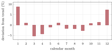
Figure 23.1. The Henry Hub natural gas spot price’s seasonal profile: the average deviation of the monthly log price from its centred twelve-month average, by calendar month, January 2000 to July 2026 (EIA via FRED, series MHHNGSP). Data: s1_seasonal.gas_profile.

23.2 Turn-of-the-month and holiday effects

Definition 23.2 (Turn-of-the-month effect)

The turn-of-the-month effect is the tendency of stock market returns to be higher on the last trading day of a month and the first few days of the next than on other days; month-end flows (salaries, pension contributions and fund rebalancing invested at the start of the month) are the candidate mechanism.

The chapter’s test is built to be honest about searching. firm.seasonal lays out a stylised calendar (twelve months of 21 trading days, weeks of five days, nine holidays a year) under thirty years of firm.synthfut’s equity class (the mean of its ten index futures, 14.7% volatility a year). Two effects are planted: 8 basis points a day on the last day and first three days of each month, and 15 basis points on each day before a holiday. A hundred rules are generated (Listing 23.1): five weekdays, twelve months, 21 days of the month, twelve turn-of-the-month windows, the days before and after holidays, weeks of the month, fortnights of the year, first and last days of the month, and a few seasonal favourites (“May to October”, “December and January”). Each rule compares the mean return on its days with the mean on the others. Of the hundred, 23 overlap the turn-of-the-month days enough to carry that effect (an expected difference of at least 3 basis points), 2 carry the pre-holiday effect, and 75 carry nothing.

correction (5%)	turn-of-month rules found	pre-holiday rules found	rules with no effect found
none	19 of 23	0 of 2	8 of 75
Bonferroni	6	0	0
Holm	6	0	0
Benjamini–Hochberg	11	0	3
Benjamini–Yekutieli	6	0	0

The turn of the month, planted on 48 days a year, is found by every correction: its best rule, the last day and first three days, has $t = 4.4$ (Figure 23.2). The pre-holiday effect, on nine days a year, has $t = 1.5$ : real, larger per day, and invisible, because nine days a year for thirty years is 270 observations. Without correction the search reports eight false effects, among them two weekdays, three days of the month, a week of the month and two fortnights, each of which would make a paper’s table; Benjamini–Hochberg, which controls the share of false discoveries rather than the chance of any, keeps three of them; the family-wise corrections keep none. Book 4, chapter 12 derived the corrections; here they decide what a researcher believes.

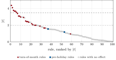
Figure 23.2. A hundred calendar rules tested on thirty years of the synthetic equity class with two planted effects: the absolute t-statistic of each rule, ranked, by what it carries. The lower dashed line is the uncorrected 5% threshold (1.96), the upper one Bonferroni’s for a hundred tests (3.48). Data: s1_seasonal.calendar_test.

23.3 Same-month seasonality in stock returns

Heston and Sadka found a pattern in the cross-section: stocks with high returns in a calendar month tend to have high returns in the same calendar month in later years, at annual lags of up to twenty years, independent of size, industry, earnings announcements, dividends and fiscal year. The signal is simple: a stock’s average return in the same calendar month of past years. The chapter plants it in firm.synthmkt: each listing receives a return for each calendar month, the same every year, with a cross-sectional standard deviation of 1% a month, spread over the month’s days.

The signal, averaged over the previous five years, has a monthly rank IC of 0.031 with the month’s return ( $t = 3.8$ over 108 months); a decile long–short earns 0.50% a month at a Sharpe ratio of 0.72, before costs. The planted effect is small against a monthly specific volatility of several percent, and the signal averages only five past observations of it. A true, stable seasonal effect is a weak signal because each stock shows it once a year.

23.4 What survives out of sample

Sullivan, Timmermann and White titled their study of calendar effects “dangers of data mining”, and the chapter’s experiment shows the danger in miniature: eight false discoveries out of a hundred rules, three even under a false-discovery-rate control. What survives has three things. A mechanism that says why the days differ (month-end flows, storage, heating), stated before the test. A test that counts every rule tried, including those that were looked at and dropped. And enough observations: an effect on nine days a year needs about half a century to reach a t-statistic of 3.48 at the chapter’s size. Most published calendar effects fail at least one of the three.

23.5 Strategy files

Strategy file 23.1 — Natural-gas seasonal spread

Who pays you, and why. Hedgers of winter demand who pay a premium for winter delivery beyond the expected seasonal price.

Instruments and venues. Natural-gas futures for winter and summer delivery.

Signal. The winter–summer spread against storage levels and its own history.

Sizing and execution. Spread positions, small; rolled with the strip.

Costs. Moderate; wide spreads in far months.

How it dies. Cold winters: the risk it is paid for.

Horizon, capacity, infrastructure. Months; storage and weather data.

Backtest honestly. Futures prices, not the spot’s seasonal profile; storage data as released.

Sources. No performance figure verified; the spot profile from EIA data.

Strategy file 23.2 — Turn-of-the-month

Who pays you, and why. Month-end and month-start flows that buy equities on predictable days.

Instruments and venues. Equity index futures.

Signal. The calendar: the last trading day and the first three.

Sizing and execution. Long on those days, flat otherwise; or tilt an existing book’s exposure.

Costs. Two round trips a month.

How it dies. Arbitrage of a published pattern; changes in payroll and fund-flow timing.

Horizon, capacity, infrastructure. Days; large capacity in index futures.

Backtest honestly. The exact window fixed before the test; every window tried counted.

Sources. Lakonishok and Smidt (1988); this chapter: found by every correction when planted at 8 basis points a day.

Strategy file 23.3 — Same-calendar-month seasonality

Who pays you, and why. Recurring annual flows and events specific to each firm.

Instruments and venues. Stocks.

Signal. A stock’s average return in the same calendar month of past years.

Sizing and execution. Monthly decile or rank long–short, neutral to factors.

Costs. A full rebalance every month.

How it dies. Crowding; the costs of a monthly turnover.

Horizon, capacity, infrastructure. A month; long return histories.

Backtest honestly. Delisted stocks included; lags of whole years only.

Sources. Heston and Sadka (2008); this chapter: IC 0.031, 0.50% a month decile spread before costs.

Strategy file 23.4 — Pre-holiday effect

Who pays you, and why. Unclear: mood and short covering before a closure are the usual stories.

Instruments and venues. Equity index futures.

Signal. The trading day before an exchange holiday.

Sizing and execution. Long for the day.

Costs. One round trip per holiday.

How it dies. It may never have lived: few observations a year.

Horizon, capacity, infrastructure. A day.

Backtest honestly. The holiday calendar as it was each year; enough years for nine events a year to mean something.

Sources. Lakonishok and Smidt (1988); this chapter: $t = 1.5$ in thirty years when planted at 15 basis points.

23.6 Tutorial: a handful survive

Goal. Generate a hundred calendar rules, test them on a synthetic market with two planted effects, correct four ways and count true and false discoveries; test same-month seasonality in the cross-section; read the seasons of natural gas and crude oil. End state: the table and the two figures.

Rules and their test.

def rules(cal):
    out = [(f"weekday {k}", cal["dow"] == k) for k in range(DPW)]
    out += [(f"month {k + 1}", cal["moy"] == k) for k in range(MPY)]
    out += [(f"day {k + 1} of month", cal["dom"] == k) for k in range(DPM)]
    for last in (1, 2, 3):
        for first in (1, 2, 3, 4):
            out.append((f"turn of month -{last}..+{first}", (cal["dom"] >= DPM - last) | (cal["dom"] < first)))
    out += [("pre-holiday", cal["pre"]), ("post-holiday", cal["post"])]
    out += [(f"week {k + 1} of month", np.minimum(cal["dom"] // DPW, 3) == k) for k in range(4)]
    fortnight = (cal["moy"] * DPM + cal["dom"]) // 10
    out += [(f"fortnight {k + 1}", fortnight == k) for k in range(int(fortnight.max()) + 1)]
    out += [(f"last {k} days of month", cal["dom"] >= DPM - k) for k in range(1, 6)]
    out += [(f"first {k} days of month", cal["dom"] < k) for k in range(1, 6)]
    out += [("first half of month", cal["dom"] < DPM // 2), ("second half of month", cal["dom"] >= DPM // 2)]
    out += [("quarter-end month", cal["moy"] % 3 == 2), ("quarter-start month", cal["moy"] % 3 == 0),
            ("first half of year", cal["moy"] < 6), ("May to October", (cal["moy"] >= 4) & (cal["moy"] <= 9)),
            ("December and January", (cal["moy"] == 11) | (cal["moy"] == 0)),
            ("summer", (cal["moy"] >= 5) & (cal["moy"] <= 7))]
    return out


def score_rules(r, rule_list):
    r = np.asarray(r, float)
    names, ts = [], []
    for name, m in rule_list:
        a, b = r[m], r[~m]
        se = math.sqrt(a.var(ddof=1) / len(a) + b.var(ddof=1) / len(b))
        names.append(name)
        ts.append((a.mean() - b.mean()) / se)
    t = np.array(ts)
    p = np.array([math.erfc(abs(x) / math.sqrt(2)) for x in t])
    return names, t, p

Listing 23.1. A hundred calendar rules and the Welch test of each. code/firm/seasonal/firm_seasonal.py

The experiment: planting, testing, correcting, and classing each discovery by what it carries.

def calendar_test(seed: int = 7):
    F = simulate_futures(FutConfig(seed=seed))
    eq = F["r"][:, F["cls"] == 0].mean(1)
    cal = calendar(30)
    tom = np.where((cal["dom"] >= DPM - 1) | (cal["dom"] < 3), TOM, 0.0)
    pre = np.where(cal["pre"], PRE, 0.0)
    R = rules(cal)
    names, t, p = score_rules(eq + tom + pre, R)
    e_tom = np.array([tom[m].mean() - tom[~m].mean() for _, m in R])
    e_pre = np.array([pre[m].mean() - pre[~m].mean() for _, m in R])
    family = np.where(np.abs(e_tom) >= 3e-4, "tom", np.where(np.abs(e_pre) >= 3e-4, "pre", "none"))
    out = {"n_rules": len(R), "family": family, "names": names, "t": t, "p": p}
    for label, fn in CORRECTIONS:
        k = fn(p) < 0.05
        out[label] = {f: int((k & (family == f)).sum()) for f in ("tom", "pre", "none")}
        out[label]["false"] = [names[i] for i in np.flatnonzero(k & (family == "none"))]
    return out

Listing 23.2. The calendar experiment. code/strategies-1/23-seasonality-and-calendar-effects/python/s1_seasonal.py

Run calendar_test(), same_month_test(), wti_months() and gas_profile(), and fig_seasonal.py.

What to change next. Run the experiment on fifty seeds and count how often each correction finds the pre-holiday effect; add a rule family per year of history and watch the false discoveries grow; plant a same-month effect that fades over time.

23.7 Build: calendar rules

Purpose. A stylised calendar, a rule generator, a rule tester, seasonal profiles and the same-month signal.

Interface. calendar(years, holidays), rules(cal), score_rules(r, rules), profile(x, period), same_month(M, lags).

Rules. Every rule generated is tested and counted; the same-month signal uses whole-year lags only.

Acceptance tests. code/firm/seasonal/tests/: the calendar’s shape and the hundred distinct rules, a planted day found with the right p-value, profiles and the same-month signal by hand.

Stretch. Real exchange calendars; bootstrap (max-statistic) corrections for correlated rules; seasonal decomposition of futures curves.

Sources and further reading

S. L. Heston and R. Sadka, “Seasonality in the cross-section of stock returns”, Journal of Financial Economics 87(2), 2008.
J. Lakonishok and S. Smidt, “Are seasonal anomalies real? A ninety-year perspective”, Review of Financial Studies 1(4), 1988.
R. Sullivan, A. Timmermann and H. White, “Dangers of data mining: the case of calendar effects in stock returns”, Journal of Econometrics 105(1), 2001.
US Energy Information Administration: Henry Hub natural gas spot price (via FRED) and NYMEX WTI crude oil futures settlements.

23.8 Exercises

Exercise 23.1 ★

A hundred rules with no effect are tested at 5%. How many false discoveries do you expect? With 75 rules that carry nothing?

Solution

Solution of Exercise 23.1.

$100 \times 0.05 = 5$ ; with 75 null rules, $75 \times 0.05 = 3.75$ . The experiment found 8, within the noise of correlated rules (a false weekday tends to bring false days and fortnights with it).

Exercise 23.2 ★

What two-sided threshold does Bonferroni’s correction set for a hundred tests at 5%?

Solution

Solution of Exercise 23.2.

$\Phi^{-1}(1 - 0.05/200) = 3.48$ .

Exercise 23.3 ★

Why is the natural-gas spot price’s winter premium not a trading strategy?

Solution

Solution of Exercise 23.3.

Nobody can buy January gas in July and hold it as spot; the tradeable instruments are futures, whose prices for winter delivery already include the expected winter premium. A futures position earns only the difference between the realised and the priced season, plus any risk premium.

Exercise 23.4 ★★

Daily volatility is $14.7\%/\sqrt{252}$ . What standard error does a difference of means have for 1 440 turn-of-month days against 6 120 others, and what t-statistic does 8 basis points give? The same for 270 pre-holiday days against 7 290 others and 15 basis points?

Solution

Solution of Exercise 23.4.

Daily volatility is $0.147/\sqrt{252} = 0.93\%$ . For the turn of the month the standard error is $0.93\% \times \sqrt{1/1\,440 + 1/6\,120} = 2.71$ basis points, so 8 basis points give $t = 2.95$ on average (the sample drawn gave 4.4). For holidays it is $0.93\% \times \sqrt{1/270 + 1/7\,290} = 5.74$ basis points and $t = 2.61$ (the sample gave 1.5).

Exercise 23.5 ★★

How many years would the pre-holiday effect need for its expected t-statistic to reach 3.48?

Solution

Solution of Exercise 23.5.

The t-statistic grows with the square root of the sample: $30 \times (3.48/2.61)^2 = 53$ years.

Exercise 23.6 ★★

Why does Benjamini–Hochberg keep false discoveries that Bonferroni rejects, and when is that acceptable?

Solution

Solution of Exercise 23.6.

It controls the expected share of false discoveries among those made, not the chance of making any; with many true effects it keeps more of them and tolerates a few false ones. That is acceptable when discoveries feed further tests (a research pipeline), not when each is traded as found.

Exercise 23.7 ★★★

Coding. Change the seed of simulate_futures in calendar_test to 8 and rerun. Which results change, and which do you expect to stay?

Solution

Solution of Exercise 23.7.

With seed 8 the best turn-of-month rule has $t = 2.25$ and the pre-holiday rule $t = 2.99$ : uncorrected, 8 turn-of-month rules, the pre-holiday rule and 4 rules that carry nothing are found; every correction finds nothing. The planted effects did not change; the sample did. What should stay is the pattern of the corrections (few or no false discoveries); what changes is which true effects are lucky enough to pass.

Exercise 23.8 ★★★

Find the flaw. “Mondays have been negative in our data at $t = 2.4$ ; we short index futures every Monday.”

Solution

Solution of Exercise 23.8.

Mondays are one of many calendar rules anyone has looked at; $t = 2.4$ does not survive a correction for them. A mechanism, an out-of-sample period and the costs of 52 round trips a year are needed before trading it.

23.9 Problem: A Handful Survive

Problem 23.1

Weekend problem — a hundred calendar rules

The chapter’s synthetic markets, the EIA data and the public record.

Part I — Seasons.

Define a calendar effect, the turn-of-the-month effect and return seasonality.
Give natural gas’s seasonal profile and explain it.
What did the WTI test by calendar month find?
What did Lakonishok and Smidt find?

Part II — The experiment.

Describe the calendar, the planted effects and the hundred rules.
How are rules classed as carrying an effect or nothing?
Give the discoveries at each correction.
Why is the pre-holiday effect never found?

Part III — The cross-section.

What did Heston and Sadka find?
Describe the planted same-month effect and the signal.
Give its IC and the decile spread.
Why is a stable seasonal effect a weak signal?

Part IV — The verdict.

State the named result: the planted effects found and the false discoveries at each correction.
List the three things a surviving calendar effect has.
Which correction would you use for a search of a hundred rules, and why?
How would you backtest a turn-of-the-month strategy honestly?
What does “dangers of data mining” refer to?
Which strategy file has the weakest mechanism?
How does this chapter relate to Book 4, chapter 12?
In one sentence: which calendar effects deserve belief?

Solution

Solution of Problem 23.1.

A return difference on calendar-defined days; higher returns on the last and first days of the month; recurrence of relative returns at the same point of each year.
$+8.8\%$ in January, $+7.3\%$ in December, $-5.3\%$ in March and $-4.2\%$ in April against trend: winter heating, spring refilling.
October and November lowest ( $t = -1.71$ , $-2.17$ ), nothing after correction (smallest adjusted p-value 0.36).
Persistently anomalous returns around the turn of the week, month and year and around holidays, over ninety years.
Twelve 21-day months, nine holidays, thirty years; 8 basis points on four turn-of-month days, 15 on pre-holiday days; a hundred rules.
By their expected difference from each planted effect: at least 3 basis points carries it.
None: 19 turn-of-month, 0 pre-holiday, 8 false; Bonferroni, Holm and Benjamini–Yekutieli: 6, 0, 0; Benjamini–Hochberg: 11, 0, 3.
Nine days a year give 270 observations in thirty years: an expected t of 2.6, 1.5 in this sample.
Stocks’ relative returns recur in the same calendar month for up to twenty annual lags.
A 1% monthly seasonal return per stock; the average return in the same month of the previous five years.
A rank IC of 0.031 ( $t = 3.8$ ); a decile spread of 0.50% a month, Sharpe ratio 0.72 before costs.
Each stock shows it once a year, against a monthly noise of several percent.
Named result. The turn-of-the-month effect is found under every correction (6 rules under the family-wise ones, 11 under Benjamini–Hochberg), the pre-holiday effect under none; false discoveries number 8 uncorrected, 3 under Benjamini–Hochberg and 0 under Bonferroni, Holm and Benjamini–Yekutieli.
A mechanism stated first, a test that counts every rule tried, and enough observations.
A family-wise correction (Holm) for a search to be traded directly; the false discovery rate for a screen followed by more tests.
The window fixed in advance, every window tried reported, futures prices and costs, an out-of-sample period.
That testing many rules on the same data finds effects that are not there.
The pre-holiday effect.
Book 4 derived the corrections; here they decide which calendar effects are believed.
Those with a mechanism that survive a correction for every rule tried.

23.10 Interview questions

Interview question 23.1 ★ researcher

You find that Fridays have been positive at $t = 2.2$ . What do you do next?

Solution

Solution of Interview question 23.1.

Count how many calendar rules have been tried (by me and by the literature), correct for them, look for a mechanism, check other markets and periods, and estimate what it would earn after costs; most likely, file it.

Interview question 23.2 ★★ researcher

What is the difference between controlling the family-wise error rate and the false discovery rate?

Solution

Solution of Interview question 23.2.

The family-wise error rate is the probability of at least one false discovery; the false discovery rate is the expected share of discoveries that are false. The first is stricter; the second keeps more true effects when there are many.

Interview question 23.3 ★★ trader

Why might month-end flows move equity prices, and how would you check?

Solution

Solution of Interview question 23.3.

Salaries, pension contributions and fund inflows arrive around month-end and are invested within days; index funds rebalance at month-end. Check fund flow data by day of month and whether the effect is larger where such flows are larger.

Interview question 23.4 ★★ developer

What must a calendar in a backtesting system get right?

Solution

Solution of Interview question 23.4.

Each exchange’s trading days and holidays, as they were each year; early closes; expiry and settlement dates; time zones; and the mapping of events known in advance from those announced later.

Interview question 23.5 ★★ researcher

How is seasonality in a commodity’s spot price different from seasonality in its futures returns?

Solution

Solution of Interview question 23.5.

Spot seasonality is predictable and priced into the futures curve, so futures returns need not be seasonal; seasonality in futures returns is a risk premium or a mispricing, and much harder to find.

Interview question 23.6 ★★★ researcher

A rule’s days are a fraction $f$ of $n$ days, the effect is $\delta$ per rule day and daily volatility is $\sigma$ . Derive the expected t-statistic of the difference of means and the number of days needed for it to reach $z$ .

Solution

Solution of Interview question 23.6.

The difference of means has standard error $\sigma\sqrt{1/(fn) + 1/((1 - f)n)} = \sigma/\sqrt{f(1 - f)n}$ , so $E[t] = \delta\sqrt{f(1 - f)n}/\sigma$ ; it reaches $z$ when $n = z^2\sigma^2/(\delta^2 f(1 - f))$ .

Terms defined in this chapter

See all 2333 terms in the glossary