Derivatives and Volatility · Derivatives

1No Arbitrage and the Fundamental Theorems

Four S&P 500 index options sit in one order: a call bought and a call sold, a put sold and a put bought, at the strikes 5 000 and 6 000, all expiring in a year. Whatever the index does, the four together pay exactly 1 000 index points at expiry, USD 100 000 per set of contracts. The package trades at 958.90 points. Nobody on the desk thinks of it as an option position: it is a one-year zero-coupon bond, guaranteed by the clearing house, and 958.90 is an interest rate of 4.20%. Some funds lend cash this way, others borrow; the exchange publishes the market’s size. Behind the trade sits the idea on which every chapter of this book rests: two portfolios with the same payoff must have the same price, or someone takes the difference for nothing. This chapter makes the idea precise, turns it into prices of states of the world, and proves the two theorems that tell us when a price is forced and when it is only bounded.

1.1 Arbitrage and the law of one price

Fix a date $0$ , a date $T$ , and a finite set of states $\omega_1,\dots,\omega_S$ , one of which will occur at $T$ . There are $N$ traded assets. Asset $j$ costs $p_j$ today and pays $D_{sj}$ in state $s$ : the market is the price vector $p\in\R^N$ and the $S\times N$ payoff matrix $D$ . A portfolio $\theta\in\R^N$ (positive entries bought, negative sold) costs $p\cdot\theta$ and pays the vector $D\theta$ .

Definition 1.1 (Contingent claim and replication)

A contingent claim is a payoff at $T$ that depends on the state: a vector $g\in\R^S$ in the one-period model, a random variable $g(S_T)$ or $g(S_t, t\le T)$ in general. A replicating portfolio for $g$ is a portfolio of traded assets whose payoff equals $g$ in every state: $D\theta = g$ .

Definition 1.2 (Arbitrage)

An arbitrage is a portfolio that costs nothing or less, never pays a negative amount, and is not identically worthless: $p\cdot \theta\le0$ , $D\theta\ge0$ , and at least one of the inequalities strict ( $p\cdot \theta<0$ , or $D\theta\ne0$ ). The market has no arbitrage when no such portfolio exists.

Definition 1.3 (Law of one price)

The law of one price holds when two portfolios with the same payoff have the same cost: $D\theta=D\theta'$ implies $p\cdot \theta=p\cdot\theta'$ . Under it, every replicable claim has a unique price, the cost of any of its replicating portfolios.

No arbitrage implies the law of one price (if two portfolios with equal payoffs had different costs, buying the cheap one and selling the dear one would be an arbitrage), but not the converse: a market in which an asset paying $(1,0)$ costs zero satisfies the law of one price and still gives something for nothing (Exercise 1.4). Arbitrage is the stronger and the useful notion: a desk that finds one executes it in size until the prices move.

Definition 1.4 (Box spread)

A box spread with strikes $K_1<K_2$ and one expiry is a long call and a short put at $K_1$ together with a short call and a long put at $K_2$ . At expiry it pays $K_2-K_1$ in every state, so its price is $P(0,T)(K_2-K_1)$ and it is a zero-coupon bond.

The first two legs are a synthetic long forward at $K_1$ , the last two a synthetic short forward at $K_2$ ; the difference of two forwards on the same asset is a sure amount (Figure 1.1). The argument is put–call parity (One Quant Book 1, chapter 25) applied twice, and like parity it needs European exercise: with American options the short legs can be assigned early and the box stops being a bond.

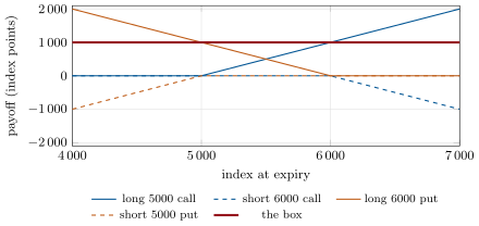
**Figure 1.1.** The four legs of a 5 000–6 000 box spread at expiry. Each leg has its kink at its strike; the calls’ kinks and the puts’ kinks cancel, and the sum is the flat line at 1 000 points. Data: the chapter’s code.

Example 1.5 (Reading the rate off a box)

The one-year 5 000–6 000 box of the opening trades at 958.90 points. Its continuously compounded rate is $-\ln(958.90/1000)=4.20\%$ . A lender who buys it pays USD 95 890 and receives USD 100 000 in a year (the multiplier is USD 100 per point); a borrower sells it.

As of September 2026 — The index box-spread market

The exchange that lists the S&P 500 index options reports USD 929 million of average daily notional volume in index box spreads in 2024. Boxes are mostly built on 1 000-point strike distances, a USD 100 000 notional per box, and the exchange describes their rates as typically 10 to 55 basis points above three-month Treasury yields. Every leg is cleared, so the lender’s counterparty is the options clearing house, not the borrower.

1.2 State prices in one period

Definition 1.6 (Arrow–Debreu security and state price)

The Arrow–Debreu security of state $s$ pays 1 if state $s$ occurs and nothing otherwise. Its price $q_s$ is the state price of $s$ . A vector $q\in\R^S$ is a state-price vector for the market if it prices every traded asset: $p = D^\top q$ , that is $p_j=\sum_s q_sD_{sj}$ .

If the Arrow–Debreu securities traded, every claim $g$ would be the portfolio $\sum_s g_s$ units of security $s$ , and would cost $q\cdot g$ . They do not trade, but state prices can still exist: they are the unknowns of the linear system $D^\top q=p$ , one equation per asset.

Theorem 1.7 (No arbitrage and positive state prices)

In the one-period finite model there is no arbitrage if and only if there is a state-price vector with $q_s>0$ for every state.

Proof. If $q>0$ prices every asset and $D\theta\ge0$ , then $p\cdot\theta=q\cdot D\theta\ge0$ , with equality only if $D\theta=0$ : no portfolio is an arbitrage. Conversely, suppose there is no arbitrage. The set $C=\{(-p\cdot\theta, D\theta):\theta\in\R^N\}$ is a linear subspace of $\R^{1+S}$ that meets the non-negative orthant only at zero. By the separating hyperplane theorem (Farkas’ lemma, One Quant Book 4, chapter 23) there is a vector $(\phi_0,\phi)$ with strictly positive entries orthogonal to $C$ : $-\phi_0\,p\cdot\theta+\phi\cdot D\theta=0$ for all $\theta$ . Then $q=\phi/\phi_0>0$ satisfies $p=D^\top q$ . ∎

State prices carry two familiar objects. If a riskless bond paying 1 in every state trades, its price is $\sum_sq_s=P(0,T)$ , and the normalised $\pi_s=q_s/P(0,T)$ are positive weights summing to one: a probability, under which every asset’s price is its discounted expected payoff, $p_j=P(0,T)\sum_s\pi_sD_{sj}$ . That probability is the risk-neutral measure of One Quant Book 4, chapter 5, the equivalent martingale measure with the bank account as numeraire: prices divided by the bond are martingales. Nothing in it says that states are likely or unlikely; it is a normalisation of prices.

Definition 1.8 (State-price density)

Given the real-world probabilities $\P(s)>0$ of the states, the state-price density is $m_s=q_s/\P(s)$ ; every price is an expectation under $\P$ : $p_j=\E[mD_j]$ . It is the ratio of the risk-neutral to the real-world probability times the discount factor, and it is high in the states in which investors most value a payoff.

Example 1.9 (A binomial market)

A bond costs 0.98 and pays 1; a share costs 100 and pays 120 or 90. The equations $q_u+q_d=0.98$ and $120q_u+90q_d=100$ give $q_u=0.3933$ , $q_d=0.5867$ , both positive: no arbitrage. The risk-neutral probability of the up state is $0.3933/0.98=0.4014$ , whatever its real-world probability. A call struck at 100 pays $(20,0)$ and is worth $20q_u=7.8667$ .

1.3 Martingale measures and the first fundamental theorem

Over several periods, a portfolio is rebalanced at each date $t_k$ according to what is known then. Let $S_t$ be the vector of risky prices, $B_t$ the bank account, and $\theta_k$ the holdings chosen at $t_k$ and kept until $t_{k+1}$ .

Definition 1.10 (Self-financing strategy)

A trading strategy $(\theta_k)$ , adapted to the information available at each date, is a self-financing strategy if nothing is added or withdrawn between $0$ and $T$ : every rebalancing is paid for by the portfolio itself, so its value changes only through price changes, $V_{t_{k+1}}-V_{t_k}=\theta_k\cdot(S_{t_{k+1}}-S_{t_k})$ in discounted units. In continuous time, $dV_t=\theta_t\,dS_t$ with a stochastic integral.

An arbitrage over several periods is a self-financing strategy with $V_0\le0$ , $V_T\ge0$ and $\P(V_T>0)>0$ (or $V_0<0$ ). The one-period result extends date by date.

Theorem 1.11 (Fundamental theorem of asset pricing)

In a market with finitely many trading dates, the fundamental theorem of asset pricing states that there is no arbitrage if and only if there exists an equivalent martingale measure: a probability $\mathbb Q$ equivalent to $\P$ under which every discounted price $S_t/B_t$ is a martingale. The arbitrage-free price of a claim $g$ paid at $T$ is then $B_0\E^{\mathbb Q}[g/B_T]$ for such a $\mathbb Q$ .

Proof. Admitted here. ∎

For a finite state space the proof is the one-period theorem applied on every node of the information tree, the state prices of each node giving the conditional probabilities of $\mathbb Q$ (Harrison and Kreps, then Harrison and Pliska). For general discrete time it is due to Dalang, Morton and Willinger; in continuous time “no arbitrage” must be strengthened to “no free lunch with vanishing risk” and the martingale property weakened to a sigma-martingale (Delbaen and Schachermayer); the measure-theoretic statements and Girsanov’s theorem, which builds $\mathbb Q$ in diffusion models, are in One Quant Book 4, chapters 1 and 5. What the desk needs is the direction of use: to price, find a measure under which discounted traded prices are martingales, and take the expectation.

Remark 1.12 (Why the bank account)

Nothing forces the bank account as unit. Any traded asset with positive price can serve as numeraire $\mathcal N_t$ : under its measure $\mathbb Q^{\mathcal N}$ prices divided by $\mathcal N_t$ are martingales. Choosing the numeraire well (the zero-coupon bond for a payoff at $T$ , the asset itself for a payoff in shares) removes a stochastic discount from an expectation; chapter 3 uses it to derive the Black–Scholes formula in two lines.

1.4 Completeness, replication and the second theorem

Definition 1.13 (Complete market)

A complete market is one in which every contingent claim has a replicating self-financing strategy. In the one-period finite model, the market is complete if and only if $D$ has rank $S$ .

Theorem 1.14 (Second fundamental theorem)

In an arbitrage-free market with finitely many dates and states, the market is complete if and only if the equivalent martingale measure is unique.

Partial proof (one period). The state-price vectors are the solutions of $D^\top q=p$ with $q>0$ . If $D$ has rank $S$ , $D^\top$ is injective and the solution is unique. If the rank is less than $S$ , the kernel of $D^\top$ contains some $z\ne0$ , and $q+\varepsilon z$ remains a positive solution for small $\varepsilon$ : the measure is not unique. ∎

A complete market prices every claim: the price is the cost of the replicating portfolio, and holding that portfolio against a sale of the claim leaves no risk. This is what makes option pricing a trade and not an opinion. The binomial market of Example 1.9 is complete; chapter 2 builds a whole pricing theory from it. Add a third state and it is not.

The trinomial market: two assets, three states. The two equations q_u+q_m+q_d=0.98 and 120q_u+100q_m+80q_d=100 leave one degree of freedom, a segment of state-price vectors whose end points each give one state a zero price. Illustrative numbers. — **Figure 1.2.** The trinomial market: two assets, three states. The two equations $q_u+q_m+q_d=0.98$ and $120q_u+100q_m+80q_d=100$ leave one degree of freedom, a segment of state-price vectors whose end points each give one state a zero price. Illustrative numbers.

1.5 Price bounds when the market is incomplete

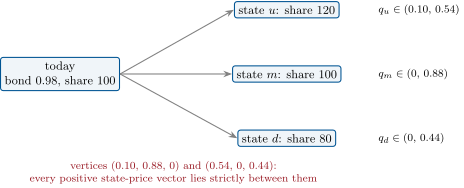
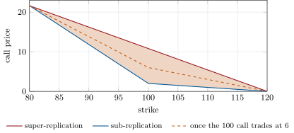
In the trinomial market of Figure 1.2 a call struck at 100 pays $(20,0,0)$ . Its price must be $20q_u$ for some positive state-price vector, so anything strictly between $20\times0.10=2$ and $20\times0.54=10.80$ is consistent with no arbitrage. The market has not chosen.

Definition 1.15 (Super-replication price)

The super-replication price of a claim $g$ is the lowest cost of a portfolio of traded assets that pays at least $g$ in every state: $\inf\{p\cdot\theta: D\theta\ge g\}$ . The sub-replication price is the highest cost of one that pays at most $g$ .

Proposition 1.16 (The no-arbitrage interval)

In an arbitrage-free one-period market, the super-replication price of $g$ equals $\max q\cdot g$ over state-price vectors $q\ge0$ with $D^\top q=p$ , and the sub-replication price equals the minimum. A new asset paying $g$ can be added at price $c$ without creating an arbitrage if and only if $c$ lies strictly between them, or $g$ is replicable and $c$ is its price.

Proof. The first statement is linear-programming duality: the dual of $\min\{p\cdot \theta:D\theta\ge g\}$ is $\max\{q\cdot g:D^\top q=p,\ q\ge0\}$ , and both optima are attained and equal when the feasible sets are non-empty. For the second, apply Theorem 1.7 to the enlarged market: a positive state-price vector exists for it exactly when $c=q\cdot g$ for some $q>0$ pricing the old assets, and the values $q\cdot g$ over the open set of positive $q$ fill the open interval (or a single point when $g$ is replicable). ∎

At the end of the interval the claim is still an arbitrage: at 10.80 the call can be sold and super-replicated at zero net cost by $0.5$ share and $-40$ bonds, and the hedged position pays $(0,10,0)$ , nothing in two states and 10 in the third. Figure 1.3 shows the interval by strike: wide at the money, where the call’s payoff depends on the state the two assets cannot tell apart, closed at the ends of the strike range, where the call is replicable.

**Figure 1.3.** The no-arbitrage interval of a call in the trinomial market, by strike. Once one option trades (the 100 call at 6.00) the market is complete and every other strike has a single price, the dashed line, inside the band. Data: the tutorial.

Method 1.17 (Static bounds on a quoted chain)

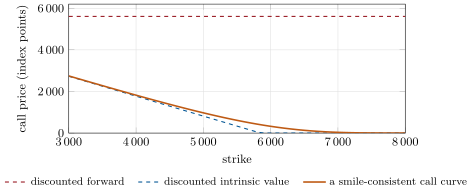
For European calls on one underlying with forward $F$ and discount factor $P$ , without any model:

$P\max(F-K,0)\le C(K)\le PF$ ; for puts $P\max(K-F,0)\le P(K)\le PK$ ;
$C$ decreases in $K$ and $C(K_1)-C(K_2)\le P(K_2-K_1)$ (the call spread pays at most the strike distance);
$C$ is convex in $K$ : a butterfly costs at least zero;
$C(K)-P(K)=P(F-K)$ at every strike, and every box costs $P(K_2-K_1)$ .

With bid and ask quotes each check is made at executable prices; a failure is an arbitrage whose portfolio the check names (Figure 1.4).

Where a call price can lie: between the discounted intrinsic value P (F-K,0) and the discounted forward PF, decreasing and convex in the strike. The solid curve is the chain of the weekend problem (forward 5 850, one year, a skewed smile). Illustrative parameters. — **Figure 1.4.** Where a call price can lie: between the discounted intrinsic value $P\max(F-K,0)$ and the discounted forward $PF$ , decreasing and convex in the strike. The solid curve is the chain of the weekend problem (forward 5 850, one year, a skewed smile). Illustrative parameters.

1.6 Tutorial: state prices, bounds and a box-spread rate

Goal. Solve for state prices, compute the no-arbitrage interval of a claim in an incomplete market, find an arbitrage portfolio when a price leaves the interval, and read a rate off a quoted box. End state: Figure 1.3 and the numbers of Example 1.9 and of the weekend problem.

Vertices of the state-price set. Every vertex solves the system on a support of as many states as there are assets; the bounds of a claim are attained at vertices.

def state_price_vertices(d: np.ndarray, p: np.ndarray, tol: float = 1e-12) -> list[np.ndarray]:
    """Vertices of {q >= 0 : D^T q = p}: basic solutions with at most (number of assets) non-zeros."""
    n_states, n_assets = d.shape
    out = []
    for support in itertools.combinations(range(n_states), n_assets):
        sub = d[list(support)].T
        if abs(np.linalg.det(sub)) < 1e-12:
            continue
        qs = np.linalg.solve(sub, p)
        if np.all(qs >= -tol):
            q = np.zeros(n_states)
            q[list(support)] = qs
            out.append(q)
    return out


def price_bounds(d: np.ndarray, p: np.ndarray, g: np.ndarray) -> tuple[float, float]:
    """No-arbitrage bounds of a claim with payoff g: min and max of q.g over state-price vectors."""
    vals = [float(q @ g) for q in state_price_vertices(d, p)]
    return min(vals), max(vals)

Listing 1.1. State-price vertices and the no-arbitrage bounds of a claim. code/derivatives/01-no-arbitrage-and-the-fundamental-theorems/python/dv_arbitrage.py

The primal side. The cheapest super-replicating portfolio, and a search for an arbitrage portfolio, are linear programmes; the build’s lp_max solves them exactly by enumerating basic solutions.

def superreplication(d: np.ndarray, p: np.ndarray, g: np.ndarray, box: float = 1e4):
    """Cheapest portfolio theta with D theta >= g: (cost, theta). Its cost is the upper bound."""
    n = d.shape[1]
    a = np.vstack([-d, np.eye(n), -np.eye(n)])
    b = np.concatenate([-g, box * np.ones(n), box * np.ones(n)])
    val, theta = lp_max(-p, a, b)
    return -val, theta


def find_arbitrage(d: np.ndarray, p: np.ndarray, bounds, eps: float = 1e-6):
    """Maximise the cash received today, -p.theta (plus eps times the total payoff, which picks up
    zero-cost arbitrages), over portfolios with D theta >= 0 and |theta_i| <= bounds[i].

    The optimum is positive exactly when an arbitrage exists; theta is then an arbitrage portfolio."""
    n = d.shape[1]
    c = -p + eps * d.sum(axis=0)
    a = np.vstack([-d, np.eye(n), -np.eye(n)])
    b = np.concatenate([np.zeros(d.shape[0]), bounds, bounds])
    val, theta = lp_max(c, a, b)
    return float(-p @ theta), theta

Listing 1.2. Super-replication and an arbitrage search as linear programmes. code/derivatives/01-no-arbitrage-and-the-fundamental-theorems/python/dv_arbitrage.py

Run the tests: the upper bound equals the super-replication cost for every strike, the call spread 90–110 has a one-point interval, and pricing the 100 call at 11.00 returns the arbitrage $(-40, 0.5, -1)$ with an edge of 0.20.

The box. Price the four legs at executable prices and invert:

def box_cost(quotes: dict[tuple[str, float], Quote], k1: float, k2: float, buy: bool = True) -> float:
    """Cash paid to buy (or received to sell) the box: long K1 call, short K2 call, short K1 put, long K2 put."""
    s = 1.0 if buy else -1.0
    legs = ((("C", k1), s), (("C", k2), -s), (("P", k1), -s), (("P", k2), s))
    cash = sum(_px(quotes[key], qty) for key, qty in legs)
    return cash if buy else -cash


def box_rate(price: float, width: float, years: float) -> float:
    """Continuously compounded rate implied by a box costing `price` that pays `width` in `years`."""
    return -math.log(price / width) / years

Listing 1.3. The cost of buying or selling a box, and the rate it implies. code/firm/arbcheck/firm_arbcheck.py

What to change next. Add a fourth state and a second option and watch the interval of a third option shrink; then quote the four box legs one tick wider and see how far the lending and borrowing rates move apart.

1.7 Build: the static-arbitrage checker

Purpose. Before any model touches a chain of quotes, the miniature firm checks that the chain itself is free of static arbitrage, and reports the portfolio and the edge of every violation. The same checks guard the surface fits of chapters 7 and 8.

Interface. Quote(strike, right, bid, ask); check_chain(quotes, forward, df) -> list[Violation] with Violation(kind, strikes, edge, legs); box_cost, box_rate, check_box; lp_max(c, a_ub, b_ub).

Rules. Buy at the ask, sell at the bid; an edge is cash received today by a portfolio whose payoff is never negative; convexity is checked on unequal strike spacing with the weights $(K_3-K_2)/(K_3-K_1)$ and $(K_2-K_1)/(K_3-K_1)$ .

Acceptance tests. code/firm/arbcheck/tests/: a Black–Scholes chain passes; a mispriced strike is caught by the convexity check with a positive edge; an option below its discounted intrinsic value is caught with the right edge; the box rate of a clean chain equals the chain’s rate.

Stretch. Replace the rule list by one linear programme over all static portfolios of the chain (options, forward, bond), which also finds violations that combine more than three strikes.

Sources and further reading

J. M. Harrison and D. M. Kreps, “Martingales and arbitrage in multiperiod securities markets”, Journal of Economic Theory 20 (1979) 381–408.
J. M. Harrison and S. R. Pliska, “Martingales and stochastic integrals in the theory of continuous trading”, Stochastic Processes and their Applications 11 (1981) 215–260.
F. Delbaen and W. Schachermayer, “A general version of the fundamental theorem of asset pricing”, Mathematische Annalen 300 (1994) 463–520.
K. J. Arrow, “The role of securities in the optimal allocation of risk-bearing”, Review of Economic Studies 31 (1964) 91–96.
J. H. van Binsbergen, W. F. Diamond and M. Grotteria, “Risk-free interest rates”, Journal of Financial Economics 143 (2022) 1–29.
Cboe, SPX box spreads (product material, 2024–2025).

1.8 Exercises

Exercise 1.1 ★

A bond costs 0.99 and pays 1; a share costs 100 and pays 115 or 95. Find the state prices, the risk-neutral probability of the up state, and the price of a call struck at 100.

Solution

Solution of Exercise 1.1.

$q_u+q_d=0.99$ and $115q_u+95q_d=100$ give $20q_u=100-94.05$ : $q_u=0.2975$ , $q_d=0.6925$ . The risk-neutral up probability is $0.2975/0.99=0.3005$ ; the call pays $(15,0)$ and is worth $15q_u=4.4625$ .

Exercise 1.2 ★

Check, for an index at expiry below 5 000, between the strikes, and above 6 000, that the 5 000–6 000 box pays 1 000 points.

Solution

Solution of Exercise 1.2.

Below 5 000: the calls pay nothing, the long 6 000 put pays $6000-S$ , the short 5 000 put costs $5000-S$ ; total 1 000. Between: the long call pays $S-5000$ , the long put $6000-S$ ; total 1 000. Above 6 000: the calls pay $(S-5000)-(S-6000)=1000$ , the puts nothing.

Exercise 1.3 ★

In the trinomial market, a put struck at 100 is offered at 9.00. Is there an arbitrage? If so, give the portfolio and its edge.

Solution

Solution of Exercise 1.3.

The put pays $(0,0,20)$ ; its interval is $(20\times0,\ 20\times0.44)=(0,\ 8.80)$ , so 9.00 is an arbitrage. Sell the put at 9.00 and super-replicate it with the portfolio that matches it in the up and down states: $-0.5$ share and 60 bonds, paying $(0,10,20)$ and costing $-50+58.8=8.80$ . The edge is 0.20 today, plus 10 in the middle state.

Exercise 1.4 ★★

Build a two-state market that satisfies the law of one price and has an arbitrage. Which of the conditions of Theorem 1.7 fails?

Solution

Solution of Exercise 1.4.

A bond paying $(1,1)$ at 0.95 and an asset paying $(1,0)$ at price 0. The payoff matrix is invertible, so each payoff has one replicating portfolio and one cost: the law of one price holds. But buying the second asset costs nothing and pays 1 in the first state: an arbitrage. The unique state-price vector is $(0,0.95)$ , not strictly positive.

Exercise 1.5 ★★

In the trinomial market completed by the 100 call at 6.00, the state prices are $(0.30, 0.48, 0.20)$ . With real-world probabilities $(0.45, 0.45, 0.10)$ , give the risk-neutral probabilities and the state-price density, and say what the density’s shape means.

Solution

Solution of Exercise 1.5.

The risk-neutral probabilities are $q/0.98$ , that is 0.3061, 0.4898 and 0.2041; the state-price density is $q/\P$ , that is 0.6667, 1.0667 and 2.0000. It is highest in the down state: a unit paid when the share has fallen is worth twice its probability-weighted value, the price of insurance against bad states.

Exercise 1.6 ★★

Give the no-arbitrage interval of a digital that pays 1 in the up state of the trinomial market, and the super-replicating portfolio at its upper end.

Solution

Solution of Exercise 1.6.

It is worth $q_u$ , strictly between 0.10 and 0.54. At 0.54 it is super-replicated by the portfolio paying $(1,0,0)$ in the up and down states: $\theta_s=1/40=0.025$ share and $-2$ bonds, which pays $(1,0.5,0)$ and costs $2.5-1.96=0.54$ .

Exercise 1.7 ★★★

Coding. With price_bounds, compute the interval of the 90–110 call spread in the trinomial market. Explain the result.

Solution

Solution of Exercise 1.7.

Both vertices give 10.80: the interval is the single point 10.80. The spread pays $(20,10,0)$ , which is $0.5$ share minus 40 bonds in every state: it is replicable, so its price is forced even though the market is incomplete.

Exercise 1.8 ★★★

Find the flaw. “In the trinomial market the 100 call can trade anywhere between 2 and 10.80. My model says it is worth 6, so I buy it at 5 and hedge: that is a riskless profit of 1.” Correct the reasoning.

Solution

Solution of Exercise 1.8.

Inside the interval no price is an arbitrage and none is “fair” without a choice of state prices: 6 is the model’s choice, not the market’s. Bought at 5, the call cannot be hedged to a sure profit, since the market cannot replicate it; the best static hedge sub-replicates it for 2 and leaves the state- $u$ risk. The profit of 1 exists only if the model’s state prices are right, which is a bet.

1.9 Problem: The Box-Spread Rate

Problem 1.1

Weekend problem — lending cash through four options

A treasurer wants to lend USD 10 million for one year through index box spreads and compares the quotes with the overnight rate, which she expects to compound to 4.00% (continuously compounded) over the year. The one-year options on the index, European and cash-settled with a USD 100 multiplier, are quoted (index points): 5 000 call 971.80–973.40, 6 000 call 324.60–326.20, 5 000 put 156.70–158.30, 6 000 put 468.40–470.00. The quotes are illustrative.

Part I — The four legs.

Write the payoff of each leg at expiry and show that the total is 1 000 points in every state.
What does one box pay in dollars?
What does the treasurer pay for one box bought leg by leg at the quotes?
What would a borrower receive for one box sold leg by leg?
Which risks does the box remove, and which remain?

Part II — Rates.

Give the lending rate implied by buying at the quotes.
Give the borrowing rate implied by selling at the quotes.
Give the mid price of the box and its rate.
How many dollars of interest does the treasurer earn per box bought leg by leg?
Give the spreads of the lending and borrowing rates over the overnight rate, in basis points.

Part III — Packages and arbitrage.

Why do boxes trade as a package at one price rather than leg by leg?
Using the overnight rate as the discount rate, is there an arbitrage in the quotes?
At what package price would the treasurer earn exactly the overnight rate?
What would change if the options were American, as single-stock options are?
Give one reason why box rates can exceed Treasury bill yields of the same maturity.

Part IV — Judgement.

Who borrows by selling boxes, and why?
How many boxes does the treasurer need, and what does she pay at the mid price?
What does she hold if the clearing member she uses defaults?
State the named result: the box’s mid implied rate and its spread over the overnight rate.
In one sentence: why is a box spread a zero-coupon bond?

Solution

Solution of Problem 1.1.

1. Long 5 000 call $(S-5000)^+$ , short 6 000 call $-(S-6000)^+$ , short 5 000 put $-(5000-S)^+$ , long 6 000 put $(6000-S)^+$ ; the calls sum to $\min(\max(S-5000,0),1000)$ and the puts to $1000-$ that amount: 1 000. 2. USD 100 000. 3. $973.40-324.60-156.70+470.00=962.10$ points, USD 96 210. 4. $971.80-326.20-158.30+468.40=955.70$ points, USD 95 570. 5. It removes all index risk; what remains is the counterparty (the clearing house), the operational risk of a leg filled without the others, and financing of the margin on a short box. 6. $-\ln(0.96210)=3.86\%$ . 7. $-\ln(0.95570)=4.53\%$ . 8. $958.90$ ; $-\ln(0.95890)=4.20\%$ . 9. $1000-962.10=37.90$ points, USD 3 790. 10. Lending $-13.6$ bp, borrowing $+53.1$ bp. 11. Legging pays half the width on each of four quotes (6.40 points in all here); a package trades at one price near the mid, and removes the risk of a partial fill. 12. The fair box is $1000e^{-0.04}=960.79$ . Buying costs 962.10, more than that, and selling brings 955.70, less: no arbitrage (check_box returns nothing). 13. 960.79 points. 14. The short legs could be assigned early, turning the box into an open position; the payoff would no longer be sure. 15. Treasuries carry a convenience yield (their use as collateral and liquidity), about 40 bp on average in the study cited, so their yield is below the riskless rate that boxes reveal. 16. Leveraged holders of index portfolios, funds and market makers who want to borrow against margin at a rate close to the riskless one rather than at a broker’s margin rate. 17. $10\,000\,000/95\,890=104.3$ : 104 boxes, paying USD 9 972 560 today and receiving USD 10 400 000 in a year. 18. Positions cleared at the clearing house, which ports them to another member or closes them out; her claim is on the clearing house, whose default resources stand behind it. 19. 4.20%, 19.7 bp above the 4.00% overnight rate. 20. Because it pays the strike distance in every state, and a sure amount at $T$ is exactly what a zero-coupon bond pays.

1.10 Interview questions

Interview question 1.1 ★ trader, researcher

What is a box spread, what does it pay, and what does its price tell you?

Solution

Solution of Interview question 1.1.

Long call and short put at $K_1$ , short call and long put at $K_2$ : two synthetic forwards that net to the sure amount $K_2-K_1$ at expiry. Its price is $P(0,T)(K_2-K_1)$ , so it quotes a riskless rate for the option’s maturity with the clearing house as counterparty; it needs European exercise.

What the interviewer is looking for: parity twice, and the rate read off the price.

Interview question 1.2 ★ researcher, bank

State the fundamental theorem of asset pricing, and say what the risk-neutral probabilities are and are not.

Solution

Solution of Interview question 1.2.

No arbitrage holds if and only if there is a probability equivalent to the real one under which discounted traded prices are martingales (in continuous time: no free lunch with vanishing risk, and a sigma-martingale). Its probabilities are normalised state prices: they encode prices, including risk premia, not beliefs about how likely states are.

What the interviewer is looking for: the equivalence, and “pricing weights, not forecasts”.

Interview question 1.3 ★★ trader

A share trades at 100 and will be at 110 or 95 in a year; the one-year rate is zero. Price a digital that pays 1 if the share ends at 110.

Solution

Solution of Interview question 1.3.

With zero rate, $110q_u+95(1-q_u)=100$ gives $q_u=1/3$ : the digital is worth 0.3333.

What the interviewer is looking for: solving for the risk-neutral probability, not using a real-world one.

Interview question 1.4 ★★ researcher

Why is a complete market equivalent to a unique martingale measure? Give an example of an incomplete market and say what happens to option prices in it.

Solution

Solution of Interview question 1.4.

State-price vectors solve $D^\top q=p$ ; the solution is unique exactly when the payoffs span every state, which is completeness. A trinomial market with a share and a bond is incomplete: option prices are only bounded, and every positive state-price vector gives an arbitrage-free price; choosing one is a model.

What the interviewer is looking for: linear algebra behind the theorem, and bounds instead of prices.

Interview question 1.5 ★★ trader, risk

Calls at strikes 90, 100 and 110 have mid prices 12.00, 6.50 and 0.90, each quoted 0.10 wide. Is there an arbitrage? What would you trade?

Solution

Solution of Interview question 1.5.

At mids the butterfly costs $12.00-13.00+0.90=-0.10$ , a convexity violation. At executable prices it costs $12.05-2\times6.45+0.95=0.10$ : no arbitrage. The mids are not tradable prices; the question is whether the quotes are.

What the interviewer is looking for: checking at bid and ask, not at mid.

Interview question 1.6 ★★★ developer

Design a service that checks 3 000 listed option quotes on one underlying for static arbitrage every time a quote changes.

Solution

Solution of Interview question 1.6.

Keep the chain sorted by expiry and strike with forward and discount factor per expiry; on each quote update recheck only the inequalities that involve the changed strike (bounds, neighbours for monotonicity and slope, the triples for convexity, the boxes through it): a constant number of checks. Use executable prices, tolerances of one tick, and debounce stale quotes; log violations with the portfolio; run a full linear-programme check periodically.

What the interviewer is looking for: incremental checks local in strike, executable prices, and a periodic global pass.

Terms defined in this chapter

See all 2333 terms in the glossary