Derivatives and Volatility · Derivatives

2The Binomial Model

The whiteboard shows a share at 100 and three steps. At each step the share goes up 10% or down 10%, and a bank deposit grows by 2%. The question is the price of a call struck at 100 that expires after the third step. There is no volatility number on the board, no probability of an up move and no formula, and the answer, 10.3603, needs none of them. Every price in this chapter is the cost of a portfolio of shares and deposit that pays exactly what the option pays, node by node; the probability that appears on the way is the one chapter 1 called risk-neutral, and it is an output of the prices, not an input. The tree is the smallest complete market in which options are non-trivial, and it is also a working pricer: with enough steps it converges to the Black–Scholes value of chapter 3, and it prices American exercise, which no closed formula does.

2.1 One period: replication and the risk-neutral probability

Definition 2.1 (Binomial model)

In the binomial model time runs in $n$ steps of length $\Delta t=T/n$ . Over each step the share price is multiplied by $u$ or by $d<u$ , and one unit of cash deposited grows to $R=e^{r\Delta t}$ (with a continuous dividend yield $q$ , the share’s own growth is compared with $e^{(r-q)\Delta t}$ ). The model has no arbitrage if and only if $d<e^{(r-q)\Delta t}<u$ .

Over one step, a claim paying $V_u$ after an up move and $V_d$ after a down move is replicated by $\Delta$ shares and a deposit $b$ if $\Delta S u+bR=V_u$ and $\Delta Sd+bR=V_d$ . Two equations, two unknowns:

\Delta=\frac{V_u-V_d}{S(u-d)},\qquad V=\Delta S+b=\frac{1}{R}\bigl(pV_u+(1-p)V_d\bigr),\qquad p=\frac{R-d}{u-d}.\tag{2.1}

The weight $p$ lies in $(0,1)$ exactly under the no-arbitrage condition; it is the risk-neutral probability of the up move, the normalised state price of chapter 1, and the real-world probability of an up move appears nowhere. Two traders who disagree about that probability agree on the price, because each can build the option from shares and cash.

Example 2.2 (One step)

A share at 50 will be at 60 or 40; rates are zero. A call struck at 50 pays 10 or 0: $\Delta=10/20=0.5$ share, and the deposit is $b=(0-0.5\times40)=-20$ , a borrowing of 20. The call costs $0.5\times50-20=5$ , and $p=(1-0.8)/0.4=0.5$ .

2.2 Many periods: the recombining tree

Definition 2.3 (Recombining tree)

A recombining tree is a tree in which an up move followed by a down move reaches the same node as the reverse: after $k$ steps the share is at one of the $k+1$ values $Su^jd^{k-j}$ , $j=0,\dots,k$ , instead of $2^k$ . Pricing on it costs $O(n^2)$ operations and $O(n)$ memory.

Applying (2.1) node by node from the last step back to the first is the backward induction of dynamic programming (One Quant Book 4, chapter 9). The portfolio at each node is rebalanced at the next using only its own value: it is a self-financing strategy in the sense of chapter 1, and it replicates the claim on every path.

Proposition 2.4 (The binomial price)

A European claim paying $g(S_T)$ after $n$ steps is worth

V_0=R^{-n}\sum_{j=0}^{n}\binom{n}{j}p^j(1-p)^{n-j}\,g\bigl(S_0u^jd^{n-j}\bigr),

the discounted expectation of the payoff when the number of up moves is binomial with parameters $n$ and $p$ .

Proof. By induction on the number of remaining steps: each backward step replaces two values by their $p$ -weighted average divided by $R$ , and the number of paths reaching node $j$ is $\binom{n}{j}$ . ∎

Figure 2.1. The whiteboard tree: share price (top line) and American put value (bottom line) at every node,

u=1.1

d=0.9

, 2% per step, strike 100. At 90 and at 81 the put is worth more exercised (10 and 19) than held (9.196 and 17.039), and the tree takes the larger value. Data: the tutorial.

Example 2.5 (The whiteboard call)

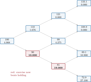
With $u=1.1$ , $d=0.9$ , $R=1.02$ : $p=(1.02-0.9)/0.2=0.6$ . After three steps the share is at 133.1, 108.9, 89.1 or 72.9, and the call pays 33.1, 8.9, 0 or 0. Its value is $(0.6^3\times33.1+3\times0.6^2\times0.4\times8.9)/1.02^3=10.3603$ . At the first node the replicating portfolio holds $\Delta=0.6240$ share and a deposit of $-52.04$ ; put–call parity holds on the tree, $C-P=100-100/1.02^3=5.7678$ .

2.3 Calibrating the tree to a volatility

To model a share with volatility $\sigma$ the step factors must reproduce, to first order in $\Delta t$ , the mean and variance of the log-return over a step. Two choices are standard; a third is built for accuracy.

Definition 2.6 (Cox–Ross–Rubinstein and Jarrow–Rudd trees)

The Cox–Ross–Rubinstein tree takes $u=e^{\sigma\sqrt{\Delta t}}$ and $d=1/u$ , so that the tree is symmetric in log-price and the drift enters only through $p$ . The Jarrow–Rudd tree takes $u,d=\exp\bigl((r-q-\tfrac12\sigma^2)\Delta t\pm\sigma\sqrt{\Delta t}\bigr)$ , which puts the drift into the factors and makes $p$ close to one half.

Proposition 2.7 (Moment matching)

In both trees the one-step log-return has risk-neutral mean $(r-q-\tfrac12\sigma^2)\Delta t+O(\Delta t^{3/2})$ and variance $\sigma^2\Delta t+O(\Delta t^2)$ , and the growth of the share matches $e^{(r-q)\Delta t}$ exactly by the choice of $p$ .

Proof. For the Cox–Ross–Rubinstein tree, expand $p=(e^{(r-q)\Delta t}-e^{-\sigma\sqrt{\Delta t}})/(2\sinh\sigma\sqrt{\Delta t})= \tfrac12+\tfrac{(r-q-\sigma^2/2)\sqrt{\Delta t}}{2\sigma}+O(\Delta t)$ ; the mean of $\pm\sigma\sqrt{\Delta t}$ is $(2p-1)\sigma\sqrt{\Delta t}$ and its second moment $\sigma^2\Delta t$ . The Jarrow–Rudd computation is the same with the drift moved into the factors. ∎

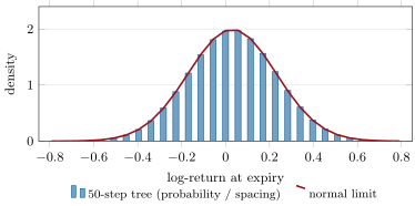
By the central limit theorem (One Quant Book 4, chapter 1) the number of up moves, centred and scaled, becomes normal: the terminal log-price of the tree converges in law to the normal distribution of geometric Brownian motion (Figure 2.2), and the tree price of a European option converges to the Black–Scholes price of chapter 3.

The risk-neutral law of the terminal log-return in a 50-step Cox–Ross–Rubinstein tree (one year, r=5\%, =20\%), each probability divided by the spacing 2 √ t between nodes, against the normal density with mean (r- 2/2)T and standard deviation √ T. Data: the tutorial. — **Figure 2.2.** The risk-neutral law of the terminal log-return in a 50-step Cox–Ross–Rubinstein tree (one year, $r=5\%$ , $\sigma=20\%$ ), each probability divided by the spacing $2\sigma\sqrt{\Delta t}$ between nodes, against the normal density with mean $(r-\sigma^2/2)T$ and standard deviation $\sigma\sqrt T$ . Data: the tutorial.

2.4 Convergence and its oscillations

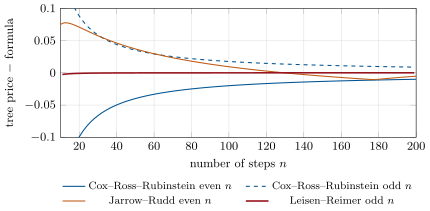
For a one-year at-the-money put with $r=5\%$ and $\sigma=20\%$ the Black–Scholes value is 5.5735. The Cox–Ross–Rubinstein price with 100 steps is 0.0200 below it, with 101 steps 0.0174 above: the error falls like $1/n$ and changes sign with the parity of $n$ (Figure 2.3). The cause is the payoff’s kink. The nodes near the strike move relative to it as $n$ changes, and the piecewise-linear payoff is sampled at a different point of its kink each time; with the strike exactly at the spot, even $n$ puts a node on the kink and odd $n$ straddles it.

Definition 2.8 (Leisen–Reimer tree)

The Leisen–Reimer tree uses an odd number of steps and chooses $p$ and $u$ so that the tree’s probabilities of finishing above the strike, under the risk-neutral and the share measures, equal $\Phi(d_2)$ and $\Phi(d_1)$ (through a normal-to-binomial inversion due to Peizer and Pratt). The tree is centred on the strike, and the error for European options falls like $1/n^2$ without oscillation.

Error of three trees for the one-year at-the-money European put (r=5\%, =20\%, formula 5.5735), even and odd step counts drawn separately. The Cox–Ross–Rubinstein error is negative for even n, positive for odd n, and shrinks like 1/n; the Leisen–Reimer error is invisible at this scale from 11 steps. Data: the tutorial. — **Figure 2.3.** Error of three trees for the one-year at-the-money European put ( $r=5\%$ , $\sigma=20\%$ , formula 5.5735), even and odd step counts drawn separately. The Cox–Ross–Rubinstein error is negative for even $n$ , positive for odd $n$ , and shrinks like $1/n$ ; the Leisen–Reimer error is invisible at this scale from 11 steps. Data: the tutorial.

Remark 2.9 (What the oscillation costs)

The Cox–Ross–Rubinstein put stays within one cent of the formula only from 199 steps on; the Leisen–Reimer tree is within 0.3 cent at 11 steps and within $10^{-4}$ at 101. Averaging the prices at $n$ and $n+1$ cancels most of the oscillation at the cost of a second tree; Richardson extrapolation (One Quant Book 4, chapter 27) removes the $1/n$ term once the oscillation is gone. Chapter 22 compares trees with finite-difference grids on accuracy against run time.

2.5 American exercise on a tree

An American option can be exercised at any node. At each node the holder compares the value of continuing, given by (2.1), with the value of exercising now, and the option is worth the larger:

V_k^j=\max\Bigl(g(S_k^j),\ R^{-1}\bigl(pV_{k+1}^{j+1}+(1-p)V_{k+1}^{j}\bigr)\Bigr).

The writer’s replicating portfolio is still self-financing where the holder continues; where the holder exercises, it is liquidated to pay the exercise value. If a holder fails to exercise at a node where exercise is optimal, the writer’s portfolio is worth more than the option from then on: the writer profits from the holder’s mistake, a theme of chapter 6.

Proposition 2.10 (No early exercise of a call without dividends)

On a tree with $r\ge0$ and $q=0$ an American call is worth the European call: exercise is never strictly optimal before expiry.

Proof. At any node the continuation value is at least $R^{-1}\bigl(pS_{k+1}^{j+1}+(1-p)S_{k+1}^{j}\bigr)-KR^{-(n-k)}$ by convexity of the payoff and induction, which equals $S_k^j-KR^{-(n-k)}\ge S_k^j-K$ : the call is worth more alive than exercised. ∎

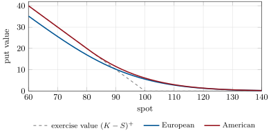
A put has no such bound: deep in the money its holder would rather have the strike now and earn interest on it (Figure 2.4). On the whiteboard tree the American put is worth 4.9076 against 4.5925 for the European: an early-exercise premium of 0.3151, earned at the two nodes of Figure 2.1 where exercise wins.

One-year puts struck at 100 (r=5\%, =20\%, 501-step Leisen–Reimer tree). The European put falls below its exercise value deep in the money, where waiting costs the interest on the strike; the American put never does, and meets the exercise value tangentially at the exercise boundary, near 81.1 here. Data: the tutorial. — **Figure 2.4.** One-year puts struck at 100 ( $r=5\%$ , $\sigma=20\%$ , 501-step Leisen–Reimer tree). The European put falls below its exercise value deep in the money, where waiting costs the interest on the strike; the American put never does, and meets the exercise value tangentially at the exercise boundary, near 81.1 here. Data: the tutorial.

2.6 Tutorial: a tree pricer and its convergence

Goal. Build the three trees, price Europeans and Americans on them, and measure their convergence to the formula. End state: Figures 2.1, 2.3 and 2.4 and the numbers of Example 2.5.

Step factors. One function returns $(u,d,p)$ for each tree and refuses a tree with an arbitrage.

def params(method: str, spot: float, strike: float, t: float, r: float, q: float, vol: float,
           n: int) -> tuple[float, float, float]:
    """(u, d, p): up and down factors per step and the risk-neutral up probability."""
    dt = t / n
    growth = math.exp((r - q) * dt)
    if method == "crr":
        u = math.exp(vol * math.sqrt(dt))
        d = 1.0 / u
    elif method == "jr":
        m = (r - q - 0.5 * vol * vol) * dt
        u, d = math.exp(m + vol * math.sqrt(dt)), math.exp(m - vol * math.sqrt(dt))
    elif method == "lr":
        if n % 2 == 0:
            raise ValueError("Leisen-Reimer needs an odd number of steps")
        s = vol * math.sqrt(t)
        d1 = (math.log(spot / strike) + (r - q) * t) / s + 0.5 * s
        p1, p = _peizer_pratt(d1, n), _peizer_pratt(d1 - s, n)
        u = growth * p1 / p
        d = (growth - p * u) / (1.0 - p)
        return u, d, p
    else:
        raise ValueError(method)
    p = (growth - d) / (u - d)
    if not 0.0 < p < 1.0:
        raise ValueError("arbitrage in the tree: need d < exp((r-q)dt) < u")
    return u, d, p

Listing 2.1. Step factors and risk-neutral probability of the three trees. code/firm/binomial/firm_binomial.py

Backward induction. One array per time slice, shortened by one at each step; American exercise is one np.maximum per slice. The dividend argument is used in chapter 5.

def price(spot: float, strike: float, t: float, r: float, vol: float, n: int, right: str = "C",
          american: bool = False, q: float = 0.0, method: str = "crr",
          dividends: tuple[tuple[float, float], ...] = ()) -> float:
    """Option value by backward induction; dividends are (time, cash amount) pairs, escrowed."""
    dt = t / n
    pv_divs = sum(a * math.exp(-r * s) for s, a in dividends if 0.0 < s <= t)
    base = spot - pv_divs
    u, d, p = params(method, base, strike, t, r, q, vol, n)
    disc = math.exp(-r * dt)
    sign = 1.0 if right == "C" else -1.0
    j = np.arange(n + 1)
    s_t = base * u ** j * d ** (n - j)
    v = np.maximum(sign * (s_t - strike), 0.0)
    for step in range(n - 1, -1, -1):
        v = disc * (p * v[1:] + (1.0 - p) * v[:-1])
        if american:
            tk = step * dt
            add = sum(a * math.exp(-r * (s - tk)) for s, a in dividends if tk < s <= t)
            j = np.arange(step + 1)
            s_k = base * u ** j * d ** (step - j) + add
            v = np.maximum(v, sign * (s_k - strike))
    return float(v[0])

Listing 2.2. Vectorised backward induction, European or American. code/firm/binomial/firm_binomial.py

Run dv_binomial.whiteboard() for the node values of Figure 2.1, then error(n, method) for $n=10,\dots,200$ and fig_binomial.py.

What to change next. Put the strike at 101 instead of 100 and watch the oscillation’s phase move; then price the American put with the average of the $n$ - and $(n+1)$ -step Cox–Ross–Rubinstein trees and compare with Leisen–Reimer.

2.7 Build: the tree pricer

Purpose. The miniature firm’s first pricer of American options, and the reference against which the finite-difference engine of chapter 22 is tested.

Interface. params(method, spot, strike, t, r, q, vol, n) -> (u, d, p) with method in crr, jr, lr; price(spot, strike, t, r, vol, n, right, american, q, method, dividends); node_values(…) for small trees.

Rules. Continuous compounding; $n$ odd for Leisen–Reimer; an arbitrage in the factors raises an error rather than returning a number; $O(n)$ memory.

Acceptance tests. code/firm/binomial/tests/: parity on the tree; convergence of all three trees to the formula; Leisen–Reimer within $10^{-4}$ at 101 steps; American call equal to European without dividends; American put above European and above its exercise value.

Stretch. A trinomial tree (chapter 22) and a pricer that returns delta and gamma from the first two time slices at no extra cost.

Sources and further reading

J. C. Cox, S. A. Ross and M. Rubinstein, “Option pricing: a simplified approach”, Journal of Financial Economics 7 (1979) 229–263.
R. J. Rendleman and B. J. Bartter, “Two-state option pricing”, Journal of Finance 34 (1979) 1093–1110.
R. A. Jarrow and A. Rudd, Option Pricing, Irwin, 1983.
D. P. J. Leisen and M. Reimer, “Binomial models for option valuation: examining and improving convergence”, Applied Mathematical Finance 3 (1996) 319–346.

2.8 Exercises

Exercise 2.1 ★

A share at 50 will be at 60 or 40; rates are zero. Give the replicating portfolio and the price of a call struck at 50, and the risk-neutral probability.

Solution

Solution of Exercise 2.1.

$\Delta=(10-0)/(60-40)=0.5$ share; the deposit $b$ solves $0.5\times40+b=0$ , so $b=-20$ (a loan). Price $0.5\times50-20=5$ ; $p=(1-0.8)/(1.2-0.8)=0.5$ .

Exercise 2.2 ★

Give $u$ , $d$ and $p$ of a one-month Cox–Ross–Rubinstein step with $\sigma=20\%$ and $r=3\%$ .

Solution

Solution of Exercise 2.2.

$u=e^{0.2/\sqrt{12}}=1.0594$ , $d=1/u=0.9439$ , $p=(e^{0.03/12}-d)/(u-d)=0.5072$ .

Exercise 2.3 ★

Check put–call parity on the whiteboard tree.

Solution

Solution of Exercise 2.3.

$C-P=10.3603-4.5925=5.7678$ and $S-KR^{-3}=100-100/1.02^3=5.7678$ .

Exercise 2.4 ★★

A colleague estimates that the share of the whiteboard goes up with probability 0.8, not 0.6, and says the call is therefore worth more than 10.3603. Explain why the price does not depend on that estimate.

Solution

Solution of Exercise 2.4.

The call is built from shares and cash, node by node, for 10.3603, and pays the call’s payoff on every path whatever the probabilities. If it traded above that, selling it and buying the portfolio would be an arbitrage; below, the reverse. The colleague’s 0.8 changes the call’s expected payoff, and equally the share’s expected return: it changes risk premia, not the price relative to the share.

Exercise 2.5 ★★

Price on the whiteboard tree a digital that pays 1 if the share ends above 100.

Solution

Solution of Exercise 2.5.

It pays at 133.1 and 108.9: $(0.6^3+3\times0.6^2\times0.4)/1.02^3=0.648/1.0612=0.6106$ .

Exercise 2.6 ★★

Compare the Cox–Ross–Rubinstein and Jarrow–Rudd factors and probabilities for $\sigma=20\%$ , $r=5\%$ , $\Delta t=0.1$ .

Solution

Solution of Exercise 2.6.

Cox–Ross–Rubinstein: $u=1.0653$ , $d=0.9387$ , $p=0.5238$ . Jarrow–Rudd: $u=1.0685$ , $d=0.9415$ , $p=0.5000$ to four decimals. The first puts the drift in the probability, the second in the factors.

Exercise 2.7 ★★★

Coding. Price the one-year at-the-money European put ( $r=5\%$ , $\sigma=20\%$ ) with 101 steps on the Cox–Ross–Rubinstein and Leisen–Reimer trees and compare both with 5.5735.

Solution

Solution of Exercise 2.7.

Cox–Ross–Rubinstein 5.5909 (0.0174 too high); Leisen–Reimer 5.5735 (error $-0.00003$ ).

Exercise 2.8 ★★★

Find the flaw. “We calibrated the tree to the data: up 5%, down 3%, and 6% growth of cash per step. The probability comes out at 1.125, but we price with it anyway.”

Solution

Solution of Exercise 2.8.

A probability of 1.125 says that cash grows faster than the share can in either state ( $R=1.06>u=1.05$ ): shorting the share and depositing the proceeds earns a riskless profit. The “calibration” describes an arbitrage, and prices computed with it are meaningless. The model requires $d<R<u$ .

2.9 Problem: The Whiteboard Tree

Problem 2.1

Weekend problem — from three steps to a working pricer

A candidate is given the whiteboard tree of this chapter (share 100, up 10%, down 10%, cash growth 2% per step, three steps, strike 100), then asked to turn it into a pricer for a one-year option with $r=5\%$ and $\sigma=20\%$ .

Part I — The European options.

Give the risk-neutral probability of an up move.
List the share prices after three steps.
Price the call.
Give the replicating portfolio at the first node.
Price the European put and check put–call parity.

Part II — American exercise.

At which nodes is early exercise of the put optimal?
Price the American put.
Give the early-exercise premium.
Is the American call worth more than the European call on this tree?
Why does the holder at the node 90 prefer exercising?

Part III — A real tree.

Give the Black–Scholes value of the one-year at-the-money put.
Give the Cox–Ross–Rubinstein errors at 100 and 101 steps.
Give the Leisen–Reimer error at 101 steps.
Price the American put with a 2 001-step Leisen–Reimer tree, and its premium.
Why does the Cox–Ross–Rubinstein error change sign with the parity of $n$ ?

Part IV — Judgement.

How many steps does each tree need for one-cent accuracy?
How does the run time grow with $n$ , and what does that imply for a desk repricing 10 000 American options?
What does a tree assume that a real market does not offer?
State the named result: the early-exercise premium on the whiteboard tree, and the number of Cox–Ross–Rubinstein steps after which the put stays within one cent of the formula.
In one sentence: why is the tree’s probability not a forecast?

Solution

Solution of Problem 2.1.

1. $p=(1.02-0.9)/0.2=0.6$ . 2. 133.1, 108.9, 89.1, 72.9. 3. 10.3603. 4. 0.6240 share and a deposit of $-52.04$ . 5. 4.5925; $C-P=5.7678=100-100/1.02^3$ . 6. At 90 after one step (10 against 9.196 held) and at 81 after two (19 against 17.039). 7. 4.9076. 8. 0.3151. 9. No: 10.3603 for both, since exercising a call early gives up the interest on the strike and the option’s remaining value. 10. Exercising pays 10 now; holding is worth 9.196 because the payoff can at best be 19 two steps later and is often less: the interest on the strike outweighs the remaining optionality. 11. 5.5735. 12. $-0.0200$ at 100 steps, $+0.0174$ at 101. 13. $-0.00003$ . 14. 6.0902; premium 0.5167 over the formula’s European value. 15. With the strike at the spot, even $n$ puts a node on the kink and odd $n$ straddles it: the discretised payoff is alternately too low and too high near the kink. 16. Cox–Ross–Rubinstein 199 steps; Leisen–Reimer 7 (every odd $n\ge7$ is within one cent). 17. As $n^2$ : 2 001 steps cost about 400 times the work of 100. For 10 000 options the desk uses the accurate tree at small $n$ , or a grid with the same work shared across strikes. 18. Two possible moves per step, continuous hedging in the limit, no costs, a known volatility: it prices by replication in a market that is not complete. 19. 0.3151 on the whiteboard; 199 steps. 20. It is the weight that makes shares and cash reproduce each other’s prices, fixed by $u$ , $d$ and $R$ , whatever anyone believes about the future.

2.10 Interview questions

Interview question 2.1 ★ trader, researcher

A share at 100 goes to 120 or 80 in one period, rates are zero. Price a call struck at 100 and give the hedge.

Solution

Solution of Interview question 2.1.

$\Delta=20/40=0.5$ share, borrow 40 (so that $0.5\times80-40=0$ ): the call costs $50-40=10$ ; $p=0.5$ .

What the interviewer is looking for: replication, not an expected value under a guessed probability.

Interview question 2.2 ★ researcher

Why does the real-world probability of an up move not enter the binomial price?

Solution

Solution of Interview question 2.2.

Because the option is replicated by shares and cash on every path; its price is the replicating portfolio’s cost. Any change in the probability changes the share’s expected return as well, and the relative price is unchanged.

What the interviewer is looking for: replication; the probability as a derived weight.

Interview question 2.3 ★★ researcher, developer

Why does the Cox–Ross–Rubinstein price oscillate as the number of steps grows, and how do you fix it?

Solution

Solution of Interview question 2.3.

The kink of the payoff sits at a different place relative to the terminal nodes for even and odd $n$ , so the sampled payoff alternates between too high and too low. Fix: Leisen–Reimer (centre the tree on the strike), average $n$ and $n+1$ , or smooth the payoff over the last step (chapter 22).

What the interviewer is looking for: the kink as the cause.

Interview question 2.4 ★★ trader

Why might you exercise an American put early, but never an American call on a share that pays no dividend?

Solution

Solution of Interview question 2.4.

A deep in-the-money put is worth nearly $K-S$ at expiry; exercising now earns interest on $K$ and gives up little optionality. For a call, exercising pays $K$ early and gives up the insurance of the optionality, while $C\ge S-Ke^{-r(T-t)}> S-K$ : it is always better sold than exercised.

What the interviewer is looking for: the interest on the strike against the value of optionality.

Interview question 2.5 ★★ developer

How many nodes does an $n$ -step recombining tree have, and how much memory does pricing on it need?

Solution

Solution of Interview question 2.5.

$(n+1)(n+2)/2$ nodes; backward induction needs only one time slice at a time, $n+1$ values, so $O(n)$ memory and $O(n^2)$ time.

What the interviewer is looking for: recombination and the one-slice array.

Interview question 2.6 ★★★ developer, researcher

Your tree pricer must return delta and gamma as well as the price, without repricing. How?

Solution

Solution of Interview question 2.6.

Read them from the nodes after one and two steps: $\Delta\approx(V_1^1-V_1^0)/ (Su-Sd)$ and gamma from the three nodes of step 2, which are centred on $S$ in a Cox–Ross–Rubinstein tree ( $Su^2$ , $S$ , $Sd^2$ ). Better, start the tree two steps before today so that the three nodes of today are $Su^2$ , $S$ , $Sd^2$ and the differences are centred.

What the interviewer is looking for: Greeks from the tree’s own nodes, centred.

Terms defined in this chapter

See all 2333 terms in the glossary