9Local Volatility

Two desks price the same forward-start put on an index: struck at 95% of wherever the index will be in six months, expiring six months later. Both use models that reproduce every listed vanilla to the tick. The first model says that six months from now the six-month smile will be little more than half as steep as it is today, and prices the put cheaply; the second says the smile will look as it does today, and charges more. Both fit today’s market; they disagree about tomorrow’s, and a forward-start option is a bet on tomorrow’s smile. The first model is local volatility: the unique diffusion whose volatility is a function of time and spot and which reprices every European option. This chapter derives it from the surface (Dupire’s formula), shows why it is the natural starting point for any smile model, calibrates it and checks it by simulation, and measures what it says about the future: the forward smile and the way the smile moves when the spot moves.

9.1 Dupire’s formula

Definition 9.1 (Local volatility model)

In a local volatility model the underlying follows

$$dS_t=(r-q)S_t\,dt+\sigma_{\mathrm{loc}}(t,S_t)S_t\,dW_t$$

under the risk-neutral measure, with a deterministic function $\sigma_{\mathrm{loc}}$, its local volatility. The model is complete: the only source of risk is the spot, and every claim is replicated with the underlying.

The Black–Scholes model is the case of a constant $\sigma_{\mathrm{loc}}$. The question is whether some function reproduces a whole surface of option prices, and which. Dupire’s answer is that exactly one does, and that it can be read off the prices.

Theorem 9.2 (Dupire’s formula)

If call prices $C(K,T)$ are smooth in $(K,T)$ and generated by a local volatility model, then

$$\sigma_{\mathrm{loc}}^2(T,K)=\frac{\partial_TC+(r-q)K\,\partial_KC+qC}{\tfrac12K^2\,\partial_{KK}C},$$

the Dupire formula. Conversely, any arbitrage-free, smooth surface of call prices determines a local volatility that reproduces it.

The numerator is the price of a calendar spread, the denominator a butterfly: local variance is the ratio of the two static arbitrages of chapter 7, and it is positive exactly when both are.

9.2 Local volatility from implied volatility

Prices are the wrong input for derivatives: they span decades of magnitude across strikes, and a second derivative of noisy prices is noise. The same formula in the coordinates of chapter 7 is better behaved.

Proposition 9.3 (Dupire in total implied variance)

With $k=\ln(K/F_{0,T})$ and $w(k,T)=\sigma_{\mathrm{imp}}^2(k,T)T$,

$$\sigma_{\mathrm{loc}}^2(T,\,F_{0,T}e^k)=\frac{\partial_Tw}{g(k)},\qquad g(k)=\Bigl(1-\frac{k\,\partial_kw}{2w}\Bigr)^2-\frac{(\partial_kw)^2}{4}\Bigl(\frac1w+\frac14\Bigr) +\frac{\partial_{kk}w}2 ,$$

where $g$ is the butterfly factor of chapter 7.

Proposition 9.4 (Local skew is twice implied skew)

For short expiries and a weak skew, the implied volatility at strike $K$ is close to the average of the local volatility between the spot and $K$; in particular the slope of the local volatility in log-strike at the money is twice the slope of the implied volatility.

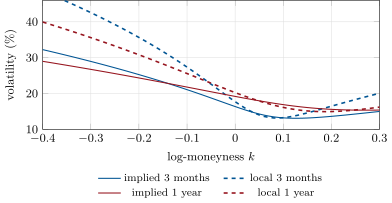
On the chapter’s surface (an SSVI surface of the kind fitted in chapter 8, with zero rates and dividends) the three-month implied volatility is 16.4% at the money and 21.1% at $k=-0.1$; the local volatility is 17.7% and 27.4%. The at-the-money slopes are $-0.47$ and $-0.92$ per unit of log-moneyness, a ratio of 1.98 (Figure 9.1).

9.3 Calibration in practice

Dupire’s formula needs the derivatives of a surface, not quotes. Three rules follow.

Method 9.5 (Building a local volatility surface)

1. Fit an arbitrage-free, smooth implied surface first (SVI or SSVI, chapter 8), with events removed and business time applied; the formula then returns a positive, finite local variance.
2. Evaluate the local volatility on a grid in time and log-moneyness against the forward of the calibration date, and interpolate it; beyond the fitted range, extrapolate flat.
3. Check the result by pricing vanillas with the local volatility model (a grid or Monte Carlo) and comparing with the surface; errors beyond the numerical noise mean the grid or the extrapolation is too coarse.

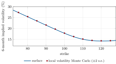
Figure 9.2 shows the check: six-month vanillas priced by 200 000 simulated paths of the local volatility model, with daily steps, return the surface’s implied volatilities to within 0.11 volatility point. The errors all have the same sign: a bias of about 0.08 point from the daily time step, since with four steps a day they fall below 0.06 point in either direction, while a four times finer grid changes them by only 0.01 to 0.02.

Local volatility is also an interpretation. Any model in which the spot has a stochastic volatility has the same one-dimensional distributions as some local volatility model.

Definition 9.6 (Markovian projection)

The Markovian projection of an Itô process $dS_t=\mu_tS_t\,dt+ \sigma_tS_t\,dW_t$, with $\sigma_t$ random, is the local volatility model with $\sigma_{\mathrm{loc}}^2(t,K)=\E\bigl[\sigma_t^2\mid S_t=K\bigr]$; by Gyöngy’s theorem, $S_t$ has the same law in both at every date.

Any smile model therefore has a local volatility: the conditional expectation of its instantaneous variance given the spot. That is how stochastic-local volatility models (chapter 20) and local correlation (chapter 17) are calibrated, and why fitting today’s vanillas says nothing about a model’s dynamics: every model that fits them has the same Markovian projection.

9.4 What local volatility predicts: dynamics and the forward smile

A local volatility model is fitted to today’s smile; everything it says about tomorrow is a consequence of that fit. Two consequences matter.

Proposition 9.7 (Smile dynamics under local volatility)

Under local volatility, when the spot falls, the implied volatility of every fixed strike rises (the smile moves towards higher strikes), and the at-the-money volatility moves, for small moves and weak skews, twice as fast as under sticky strike: $\partial\sigma_{\mathrm{ATM}}/\partial\ln S=2\,\partial\sigma_{\mathrm{imp}} /\partial\ln K$ at the money.

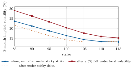
On the three-month smile of the chapter the effect is larger than the rule: a 1% fall of the index raises the at-the-money volatility 2.7 times as much as sticky strike would, a 5% fall 2.9 times, from 16.4% to 23.4% against 18.8% (Figure 9.3). The rule holds for short expiries and weak skews; the chapter’s three-month skew is neither weak nor very short. Hagan and his coauthors showed that in interest-rate markets the smile moves the other way, and that local volatility hedges were then worse than none; chapter 11 builds the model they proposed.

Definition 9.8 (Forward smile)

The forward smile from $t_1$ to $t_2$ is the implied volatility, as a function of the relative strike $x$, of forward-start options that pay $(S_{t_2}-xS_{t_1})^+$ at $t_2$: the smile that the model expects to see at $t_1$ for options of maturity $t_2-t_1$.

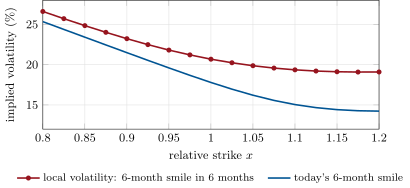
A model with time-homogeneous dynamics (the stochastic volatility models of chapter 10) produces forward smiles that resemble today’s smile of the same maturity. Local volatility does not: its local volatility function is steep near today’s spot and at short times, and flattens away from them, so the smile it generates for a future date is flatter. On the chapter’s surface the six-month smile six months forward has an at-the-money skew of $-0.19$ per unit of log-moneyness, against $-0.34$ for today’s six-month smile: 57% of it (Figure 9.4). Its level is higher (20.7% against 17.8%), which is just the term structure’s forward variance. Products whose value depends on forward skews (forward-start options, cliquets, chapter 16) are therefore priced differently by models that agree on every vanilla.

9.5 Tutorial: from a surface to a local volatility model

9.6 Build: the local volatility surface

9.7 Exercises

Exercise 9.1 ★

At some $(k,T)$ the total variance is $w=0.01$, its time derivative 0.045 and the butterfly factor $g=0.9$. Give the local volatility.

Solution

Solution of Exercise 9.1.

$\sigma_{\mathrm{loc}}=\sqrt{0.045/0.9}=\sqrt{0.05}=22.4\%$.

Exercise 9.2 ★

The three-month implied volatility is 16.4% at the money with a slope of $-0.47$ per unit of log-moneyness. Use the rule of Proposition 9.4 to estimate the local volatility at $k=-0.1$, and compare with the exact 27.4%.

Solution

Solution of Exercise 9.2.

$16.4\%+2\times(-0.47)\times(-0.1)=25.7\%$, against 27.4%: the rule captures the slope; the rest is the smile’s curvature, which the local volatility also doubles.

Exercise 9.3 ★

In a model where the spot’s volatility is 15% or 30% with equal probability, independently of the spot, what is its Markovian projection? And if, when the spot is at 90, the probability of the high state is 0.8?

Solution

Solution of Exercise 9.3.

Independent of the spot: $\sigma_{\mathrm{loc}}^2=0.5\times0.15^2+0.5\times0.30^2=0.05625$, a flat 23.7%. At 90 with probability 0.8 of the high state: $0.8\times0.09+0.2\times0.0225=0.0765$, 27.7%.

Exercise 9.4 ★★

Why must the implied surface be free of arbitrage before Dupire’s formula is applied? What does a noisy quote do to the local volatility near it?

Solution

Solution of Exercise 9.4.

The formula divides the calendar spread by the butterfly: a calendar arbitrage makes the local variance negative, a butterfly arbitrage makes the denominator negative or zero, and either gives no local volatility. A noisy quote bends the smile locally, and the second derivative in the denominator amplifies that bend into a spike or a hole in the local volatility near the quote.

Exercise 9.5 ★★

From the at-the-money total variances at six months and one year on the chapter’s surface (volatilities 17.79% and 19.19%), compute the forward at-the-money volatility from six months to one year, and compare it with the local volatility model’s forward-start at-the-money volatility, 20.68%.

Solution

Solution of Exercise 9.5.

$\sqrt{(0.1919^2\times1-0.1779^2\times0.5)/0.5}=20.49\%$, against 20.68% for the model’s forward-start at-the-money option: the level of the forward smile is essentially forward variance; the small gap is the curvature of the forward smile at the money.

Exercise 9.6 ★★

With the rule of Proposition 9.7, predict the change of the three-month at-the-money volatility after a 1% fall, and compare with the simulated 1.31 points.

Solution

Solution of Exercise 9.6.

$2\times0.47\times0.01=0.94$ point, against 1.31 simulated: the rule holds for short expiries and weak skews, and this three-month skew is steep.

Exercise 9.7 ★★★

Coding. Reprice the six-month 90 put with mc_smile using 50 000 and 200 000 paths; compare the errors with the standard errors, and say what else than Monte Carlo noise could cause an error.

Solution

Solution of Exercise 9.7.

With 50 000 paths the 90 put’s error is $-0.04$ point with a standard error of 0.13; with 200 000, $+0.11$ with a standard error of 0.06. The errors of all strikes at 200 000 paths have the same sign: a discretisation bias of the daily time step (about 0.08 point), which more paths do not remove and four steps a day does.

Exercise 9.8 ★★★

Find the flaw. “Our local volatility model reprices every listed option, so it prices every product whose payoff depends on the index at one date, including forward-start options.”

Solution

Solution of Exercise 9.8.

A European payoff on the index at one date, yes: its price depends only on the marginal distribution at that date, which the fit reproduces. A forward-start option pays on the ratio of the index at two dates, which depends on the joint distribution, and so on the model’s dynamics: local volatility gives it a flatter forward smile than a stochastic volatility model fitted to the same vanillas.

9.8 Problem: The Flattening Forward Smile

Problem 9.1

Weekend problem — what local volatility says about the smile in six months

A structurer wants to price a forward-start put struck at 95% of the index level in six months and expiring six months later, with the chapter’s surface and zero rates. The desk’s only calibrated model is local volatility.

Part I — The local volatility.

1. Give the three-month implied and local volatilities at the money and at $k=-0.1$.
2. Give the ratio of their at-the-money slopes.
3. Why is local volatility steeper than implied volatility?
4. Give the six-month repricing errors of the 80, 100 and 110 strikes.
5. What would a repricing error of one volatility point indicate?

Part II — The forward smile.

6. Give the model’s forward-start at-the-money volatility and today’s six-month at-the-money volatility.
7. Explain the difference in level with forward variance.
8. Give the at-the-money skews of the forward smile and of today’s six-month smile.
9. Give their ratio.
10. Why does local volatility flatten the forward smile?

Part III — The product.

11. Give the forward smile’s implied volatility at $x=0.95$, and the volatility that today’s six-month smile shape gives there once shifted up to the forward at-the-money level.
12. Price the forward-start put per 100 of notional with each (zero rates, Black’s formula on a forward of 1).
13. Which model would a desk that sells this put prefer, and why is that a warning?
14. What market instrument would reveal which forward skew is right?
15. How would you reserve for the model difference (chapter 27)?

Part IV — Judgement.

16. After a 5% fall of the index, what does local volatility predict for the three-month at-the-money volatility, and what does sticky strike predict?
17. When is local volatility the right model to use?
18. What must a model add to keep forward skews steep?
19. State the named result: the ratio of the local-volatility forward skew (six months in six months) to today’s six-month skew.
20. In one sentence: what does fitting every vanilla leave undetermined?

Solution

Solution of Problem 9.1.

1. 16.4% and 17.7% at the money; 21.1% and 27.4% at $k=-0.1$. 2. 1.98. 3. Implied volatility averages the local volatility between the spot and the strike; to produce a given slope of the average, the local volatility must slope twice as fast. 4. $+0.08$, $+0.06$, $+0.09$ volatility point. 5. A grid or extrapolation problem, or an arbitrage in the input surface, not noise. 6. 20.7% and 17.8%. 7. The forward at-the-money volatility from six months to one year is 20.5% from the term structure: the forward smile sits at the forward variance. 8. $-0.19$ and $-0.34$ per unit of log-moneyness. 9. 0.57. 10. Its local volatility is steep near today’s spot at short times; six months out the spot has spread and the relevant local volatilities are those of longer times, where the function is flatter. 11. 21.8%; today’s shape shifted to the forward level gives 22.5%. 12. 3.82 and 4.00 per 100. 13. Local volatility, the cheaper model for the buyer’s protection it sells; a model chosen because it prices the risk lower is a model risk (chapter 27). 14. Forward-start options or cliquets quoted by dealers, or the variance of future implied skews observed historically, which reveal how skews behave. 15. Price with both models and hold the difference, 0.18 per 100, as a model reserve until the risk is gone. 16. 23.4% under local volatility, 18.8% under sticky strike, from 16.4%. 17. For products whose value depends on the marginal distributions and short-dated dynamics (barriers near the spot, American options), and as the Markovian projection that other models are calibrated to. 18. Randomness in volatility that is not a function of the spot: stochastic volatility (chapter 10) or a forward-variance model (chapter 12). 19. 0.57: the six-month skew six months forward is 57% of today’s six-month skew. 20. The dynamics: how the smile moves with the spot and how it will look at future dates.

9.9 Interview questions

Interview question 9.1 ★ researcher

What is local volatility, and why is it unique?

Solution

Solution of Interview question 9.1.

The volatility as a deterministic function of time and spot, $\sigma_{\mathrm{loc}}(t,S)$, of a diffusion that reprices every European option. It is unique because the call prices determine the density at every date (Breeden–Litzenberger), and the density’s evolution determines the diffusion coefficient (Dupire’s formula).

What the interviewer is looking for: from prices to densities to the coefficient.

Interview question 9.2 ★ trader

The index falls. What does a local volatility model say happens to the at-the-money implied volatility, and why?

Solution

Solution of Interview question 9.2.

It rises, by about twice what sticky strike gives: the at-the-money implied volatility is close to the local volatility at the spot, which slopes twice as steeply as the implied skew, and the spot has moved to a region of higher local volatility.

What the interviewer is looking for: the factor two and its reason.

Interview question 9.3 ★★ researcher

Derive Dupire’s formula with zero rates.

Solution

Solution of Interview question 9.3.

Density $q$ solves $\partial_Tq=\tfrac12\partial_{ss}(\sigma^2s^2q)$; $C=\int(s-K)^+q\,ds$; $\partial_TC= \tfrac12\int(s-K)^+\partial_{ss}(\sigma^2s^2q)\,ds=\tfrac12\sigma^2(T,K)K^2q(T,K)$ after two integrations by parts; $q=\partial_{KK}C$. So $\sigma^2(T,K)=2\partial_TC/(K^2\partial_{KK}C)$.

What the interviewer is looking for: the forward equation and the integrations by parts.

Interview question 9.4 ★★ researcher, bank

Two models fit the same vanillas. For which products can their prices differ, and for which can they not?

Solution

Solution of Interview question 9.4.

They agree on anything that depends only on the distribution of the underlying at single dates (European payoffs, including digitals and variance swaps without jumps). They can differ on anything that depends on the joint law at several dates or on paths: barriers, Asian, lookback and forward-start options, cliquets, autocallables.

What the interviewer is looking for: marginals against joint laws.

Interview question 9.5 ★★ developer

Your local volatility surface has spikes that make the Monte Carlo pricer unstable. Where do they come from, and how do you fix them?

Solution

Solution of Interview question 9.5.

From differentiating a noisy or arbitrageable surface, from interpolation kinks between slices, and from extrapolation beyond the quoted strikes. Fit a smooth arbitrage-free parametric surface first, compute the local volatility from it in total variance, cap and floor it where the input has no information, and check by repricing.

What the interviewer is looking for: smooth input, not smoothing the output.

Interview question 9.6 ★★★ researcher, trader

What is a Markovian projection, and how would you use it to calibrate a stochastic volatility model to the whole surface?

Solution

Solution of Interview question 9.6.

The local volatility model with $\sigma^2(t,K)=\E[\sigma_t^2\mid S_t=K]$, which has the same marginals as the stochastic volatility model. To fit a stochastic volatility model to the whole surface, multiply its volatility by a leverage function $L(t,S)$ chosen so that $L^2(t,K)\,\E[\sigma_t^2\mid S_t=K]$ equals the market’s local variance: the stochastic-local volatility model of chapter 20.

What the interviewer is looking for: conditional expectation of variance given spot, and the leverage function.