Derivatives and Volatility · Derivatives
16Asians, Lookbacks, Cliquets and Forward-Starts
A corporate treasurer asks for a one-year call on the index, and then for the same call on the average of twelve monthly prices. The second quote is 40% cheaper. Nobody on the call can say where the 40% went, and the treasurer suspects a trick. There is none. The average of twelve prices moves much less than the last one: its volatility is about 61% of the index’s. This chapter prices the path-dependent payoffs that desks sell most. Asians average the path, lookbacks read its extremes, and forward-starts and cliquets are options whose strikes are set in the future. The first two are priced well by any model that fits today’s smile. The last two are not, because their value depends on the smile the model predicts for future dates. The chapter measures that dependence with two models that fit the same surface.
16.1 Averaging: Asians
Definition 16.1 (Asian option)
An Asian option pays on the average of the underlying over a set of fixing dates: the average-rate form pays (the average-price option of One Quant Book 3, chapter 12), and the average-strike form pays . The average is arithmetic unless stated.
Averaging lowers volatility. With fixings equally spaced over , the logarithm of the geometric average is normal with variance
which tends to as the fixings become continuous. The geometric Asian is therefore a Black–Scholes option at a reduced volatility and a reduced forward, in closed form. The arithmetic average, the one contracts use, has no closed form. It is larger than the geometric one, but the two move almost together.
Example 16.2 (Where the 40% went)
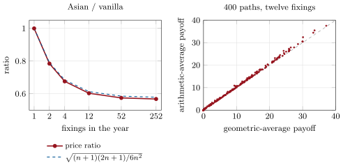
Spot and strike 100, one year, , , volatility 20%. The vanilla call is worth 8.83, and the call on the average of twelve monthly fixings is worth 5.32, 40% less. The variance factor is , so the geometric average moves with a volatility of . As the fixings multiply, the Asian’s price relative to the vanilla falls from 0.78 with two fixings to 0.68 with four, 0.60 with twelve and 0.57 with daily fixings. It tracks the volatility factor : 0.79, 0.68, 0.61 and 0.58 (Figure 16.1, left).
The near-perfect co-movement of the two averages is what makes Monte Carlo pricing of Asians cheap. The geometric Asian is a control variate (One Quant Book 4, chapter 26). Kemna and Vorst proposed it. On each path compute both payoffs, and correct the arithmetic estimate by the geometric payoff’s known error: , with estimated by regression on the same paths. On the example the two discounted payoffs have a correlation of 0.9996 and . The standard error falls from 0.025 to 0.0007, a variance reduction of 1 357 times: one path with the control variate is worth 1 357 without it (Figure 16.1, right).
Asians have two practical properties that the price alone does not show. Their risk falls as fixings pass: once half the fixings are set, half the payoff is known, and the delta and vega shrink accordingly. Hedging near a fixing, however, concentrates flow on the fixing date and time, one reason averages are taken over many fixings. And the smile’s dynamics matter little. An Asian’s value depends mostly on the at-the-money region of the smile at each fixing date, which any model fitted to the surface reproduces. On chapter 9’s surface (zero rates, twelve monthly fixings), the at-the-money Asian is worth 4.34 under local volatility and 4.36 under Heston, within one standard error of each other. Black–Scholes at the one-year at-the-money volatility gives 4.69: what matters is the term structure, since the early fixings see the lower short-dated volatilities.
16.2 Extremes: lookbacks
Definition 16.3 (Lookback option)
A lookback option pays on the maximum or minimum of the underlying over its life. The floating-strike lookback call pays (buy at the low); the fixed-strike lookback call pays .
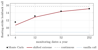
A lookback is a barrier option integrated over all barrier levels: plus the terminal price. Goldman, Sosin and Gatto priced it in closed form with the reflection principle, for continuous monitoring. It is expensive. With the example’s parameters the floating-strike lookback call is worth 15.69, 1.8 times the at-the-money call, because it buys at the best price of the year.
Contracts observe the extreme at discrete dates, often daily closes, and the monitored minimum is higher than the true one. The barrier shift of chapter 15 carries over: the monitored minimum behaves like the continuous one multiplied by , which gives with . With daily monitoring a simulation gives 15.09 (standard error 0.04) and the shifted formula 15.08. Weekly they give 14.42 and 14.34, monthly 13.13 and 12.84, and with four dates 11.55 and 10.70 (Figure 16.2). As with barriers, the correction serves daily monitoring, and a sparse schedule needs the simulation.
A lookback’s hedge is a ladder of barrier options. Each time the price makes a new low, the strike resets and the desk’s position in the option below changes. The payoff is continuous, so there is no gap at a single level, but the delta jumps each time a new extreme is set, and the vega is large. It is a volatility product more than a directional one.
16.3 Forward-starts and the forward smile
Definition 16.4 (Forward-start option)
A forward-start option is an option whose strike is fixed at a future date as a proportion of the spot then, , and which expires at . It pays for a call.
Under Black–Scholes the price follows from homogeneity. At the option is a call with strike , worth , and the expected discounted is , so the price is . It depends only on the volatility between and and on the smile that will prevail at . In any other model the implied volatilities of forward-start options across form the forward smile of chapter 9. That smile is not observed today: it is the model’s forecast.
Example 16.5 (Two forward smiles from one surface)
Chapter 9’s local volatility and chapter 10’s Heston model are both fitted to chapter 9’s surface: they reprice its one-year at-the-money call at 19.19% and 18.99% against the market’s 19.19%. Their one-month smiles starting in six months are very different (Figure 16.3). Local volatility gives 23.9% at 94%, 21.5% at the money and 21.3% at 106%, almost flat. Heston gives 24.0%, 18.5% and 20.0%, with a skew and a smile. Today’s one-month smile runs from 19.6% to 14.9% to 12.0%. Local volatility flattens the future smile, as chapter 9 found. Heston keeps its shape, and Bergomi observed that its forward smiles are more convex than today’s.
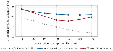
Two effects show in the example. The level is the forward volatility: the surface’s term structure rises, so the volatility from six to seven months is above today’s one-month volatility in both models. The shape is the model’s dynamics. In local volatility the skew is a function of the spot level and time, fixed at calibration, and it decays with the forward date. In Heston the skew comes from the correlation of the spot with a variance that is still random, and it is regenerated at every date. The market’s own forward smile can be read only from instruments that pay on it: forward-starts, cliquets, and the forward skew implied by options on the volatility index.
16.4 Cliquets
Definition 16.6 (Cliquet)
A cliquet (ratchet) is a series of forward-start options on consecutive periods. In its common structured form it pays the sum of the period returns , each clipped between a local floor and a local cap, with the sum clipped between a global floor and a global cap.
Definition 16.7 (Reverse cliquet)
A reverse cliquet pays a large coupon eroded by every negative period return: . The investor is short a strip of forward-start puts, capped in total.
A locally capped and floored period return is a forward-start call spread less a forward-start put spread. When the cap and floor are close to zero it behaves like a forward-start digital, and chapter 15 showed that a digital’s price is set by the skew. A cliquet is therefore a basket of bets on the forward skew, which is exactly the quantity on which the two models of the last section disagree. The reverse cliquet is short forward puts, a bet on the level of forward volatility and on how fat its left tail is.
Example 16.8 (The cliquet that fits every vanilla)
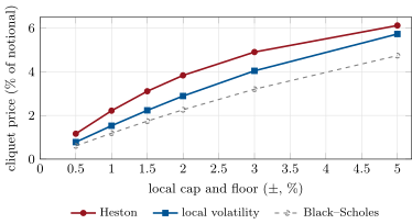
A one-year cliquet with monthly periods pays the sum of the twelve monthly returns, each clipped to , floored at zero overall. On 100 000 paths with zero rates it is worth 1.53% of notional under local volatility, 2.22% under Heston and 1.19% under Black–Scholes at the one-year at-the-money volatility. All three fit the one-year at-the-money call, and the two smile models fit the whole surface. The Heston price is 45% above the local-volatility price. The gap widens as the local cap narrows and the payoff looks more like a digital: at the prices are 0.78% and 1.16%. A reverse cliquet paying is worth 5.43% under local volatility, 7.56% under Heston and 3.57% under Black–Scholes (Figure 16.4).
In 2004 Bergomi counted reverse cliquets and Napoleons among the most recent exotic structures, and cited a review that Risk had run in February of that year under the title “Reverse cliquets: end of the road?”. His argument was that such products are priced by the dynamics a model assumes for future smiles, not by today’s surface.
16.5 Which model for which payoff
The question a structurer asks of a model is not whether it fits the surface. Local volatility, Heston with jumps, SABR by expiry and the Bergomi models all fit it, or nearly. The question is which quantities beyond the surface the payoff depends on, and whether the model’s assumptions about them are credible.
| payoff | depends on | adequate models |
|---|---|---|
| European, Asian | terminal distributions at the fixing dates | any model that fits the surface |
| barrier, lookback | the path’s extremes: the smile and its dynamics near the barrier | local or local-stochastic volatility |
| forward-start, cliquet | the forward smile, the forward skew | stochastic volatility, Bergomi |
| reverse cliquet, Napoleon | forward volatility and its volatility | Bergomi, rough models |
| options on variance or the index | the volatility of variance | forward-variance models (chapter 12) |
Bergomi’s 2004 example is the clearest statement of the principle. A six-year Napoleon paid fixed coupons for two years, then 8% a year augmented by the worst of the twelve monthly performances of the Eurostoxx 50 in each year, floored at zero. Such a product is in effect a put on long-dated forward volatility, whose value a Black–Scholes model gives without any charge for the volatility of that volatility. His “Smile dynamics II” model was built to price such products, the Napoleon and the reverse cliquet among its examples, with separate control of the short forward skew, the spot–volatility correlation and the term structure of the volatility of volatility. When two fitted models disagree by 45%, as in Example 16.8, the desk prices with the model whose dynamics it can defend and holds a reserve for the difference (chapter 27).
16.6 Tutorial: payoffs on a common path interface
Goal. Price an arithmetic Asian with a geometric control variate, a discretely monitored lookback, and a forward-start and a cliquet under three models that fit the same at-the-money volatility. End state: the four figures and the numbers of the weekend problem.
The control variate. Both payoffs on the same paths, by regression, the geometric error removed:
def asian_mc(s: float, k: float, t: float, r: float, q: float, vol: float, n: int, n_paths: int = 100_000,
             seed: int = 16, right: str = "C") -> dict:
    """Arithmetic Asian by Monte Carlo, plain and with the geometric Asian as control variate (the coefficient
    estimated by regression on the same paths)."""
    times = t * np.arange(1, n + 1) / n
    p = gbm_paths(s, times, r, q, vol, n_paths, seed)
    disc = math.exp(-r * t)
    a = disc * asian_payoff(p, k, right)
    g = disc * asian_payoff(p, k, right, geometric=True)
    exact_g = geometric_asian(s, k, t, r, q, vol, n, right)
    c = np.cov(a, g)
    beta = c[0, 1] / c[1, 1]
    adj = a - beta * (g - exact_g)
    m = len(a)
    corr = c[0, 1] / math.sqrt(c[0, 0] * c[1, 1])
    return {"plain": float(a.mean()), "plain_se": float(a.std() / math.sqrt(m)), "cv": float(adj.mean()),
            "cv_se": float(adj.std() / math.sqrt(m)), "beta": float(beta), "corr": float(corr), "geometric": exact_g}
Listing 16.1. Arithmetic Asian with the geometric control variate. code/firm/pathdep/firm_pathdep.py Payoffs read paths only. Period returns, the cliquet and the reverse cliquet:
def period_returns(paths: np.ndarray) -> np.ndarray:
    """Returns between consecutive columns: S_i / S_(i-1) - 1."""
    return paths[:, 1:] / paths[:, :-1] - 1


def cliquet_payoff(paths: np.ndarray, local_floor: float = -math.inf, local_cap: float = math.inf,
                   global_floor: float = -math.inf, global_cap: float = math.inf) -> np.ndarray:
    """Sum of the period returns, each clipped to [local_floor, local_cap], then the sum clipped globally."""
    clipped = np.clip(period_returns(paths), local_floor, local_cap)
    return np.clip(clipped.sum(axis=1), global_floor, global_cap)


def reverse_cliquet_payoff(paths: np.ndarray, coupon: float) -> np.ndarray:
    """max(0, coupon + sum of the negative period returns): the coupon is eroded by every fall."""
    return np.maximum(0.0, coupon + np.minimum(period_returns(paths), 0.0).sum(axis=1))
Listing 16.2. Cliquet payoffs on the common path array. code/firm/pathdep/firm_pathdep.py - Paths from each model:
firm_localvol.simulatewith recorded dates,firm_heston.simulate_paths,gbm_paths; then rundv_pathdep.forward_smiles(),cliquets()andfig_pathdep.py.
What to change next. Price the cliquet with Heston’s volatility of volatility halved and refit to keep the one-year skew; add a global cap of 5% and see which model’s price moves most; price a Napoleon-like coupon, 8% plus the worst monthly return, floored at zero.
16.7 Build: path-dependent payoffs
Purpose. The miniature firm’s library of path-dependent payoffs, written against one path array so that any simulator (Black–Scholes, local volatility, Heston, and chapter 23’s engine) prices any of them.
Interface. gbm_paths(s, times, r, q, vol, n_paths, seed); asian_payoff(paths, strike, right, geometric), geometric_asian, asian_mc; lookback_payoff, lookback_floating_call, lookback_shifted; forward_start_call; period_returns, cliquet_payoff(paths, local_floor, local_cap, global_floor, global_cap), reverse_cliquet_payoff; forward_smile_from_paths.
Rules. Column 0 of a path array is today’s spot; payoffs never simulate; every Monte Carlo price is reported with its standard error; control variates are used whenever a closed-form cousin exists.
Acceptance tests. code/firm/pathdep/tests/: the one-fixing geometric Asian is the vanilla and the formula matches a simulation; the control variate cuts the error tenfold at least; the lookback exceeds the vanilla and its shifted formula matches a daily simulation; the forward-start formula and a flat model’s forward smile; cliquet payoffs on hand paths.
Stretch. Moment-matching approximations for arithmetic Asians; fixed-strike lookbacks; the Napoleon.
Sources and further reading
- A. G. Z. Kemna and A. C. F. Vorst, “A pricing method for options based on average asset values”, Journal of Banking and Finance 14(1) (1990) 113–129.
- M. B. Goldman, H. B. Sosin and M. A. Gatto, “Path dependent options: buy at the low, sell at the high”, Journal of Finance 34(5) (1979) 1111–1127.
- L. Bergomi, “Smile dynamics”, Risk (September 2004); “Smile dynamics II”, SSRN 1493302.
- C. Jeffery, “Reverse cliquets: end of the road?”, Risk (February 2004) 20–22.
16.8 Exercises
Exercise 16.1 ★
Compute the volatility factor for and its limit as .
Solution
Solution of Exercise 16.1.
: . As the factor tends to .
Exercise 16.2 ★
Why is the arithmetic Asian worth more than the geometric one?
Solution
Solution of Exercise 16.2.
Path by path, the arithmetic mean of positive numbers is at least their geometric mean, and the call payoff is increasing in the average; so the arithmetic payoff dominates the geometric one on every path.
Exercise 16.3 ★
Under Black–Scholes with , what is a six-month-into-six-month at-the-money forward-start call worth relative to a six-month at-the-money call?
Solution
Solution of Exercise 16.3.
The six-month at-the-money call today is by homogeneity; the forward-start call is . The ratio is : the dividends paid before the strike is set lower the spot at which it is set.
Exercise 16.4 ★★
Show that and explain why a cliquet with a narrow local cap and floor behaves like a string of forward digitals.
Solution
Solution of Exercise 16.4.
If : . If : . If : . So the clipped return is a constant plus a call spread between and , . When is small the spread is times a digital at about : each period pays like a forward-start digital, whose price is set by the forward skew.
Exercise 16.5 ★★
Explain why the local-volatility forward smile is flatter than Heston’s in Example 16.5.
Solution
Solution of Exercise 16.5.
Local volatility fits today’s skew with a volatility that is a fixed function of spot and time; as the forward date recedes, the spot has moved and the local skew it meets is the one calibrated to decay with maturity, so the forward smile flattens. In Heston the skew comes from the correlation of the spot with a variance that is still random at the forward date: it is regenerated there, and the randomness of the variance adds curvature.
Exercise 16.6 ★★
A variance-reduction factor of 1 357 means what, in paths and in computing time, for a price wanted to 0.001?
Solution
Solution of Exercise 16.6.
The standard deviation of the plain estimator per path is about , so an error of 0.001 needs million paths; with the control variate about 47 000. Computing the geometric payoff adds little to each path, so the time falls by about the same factor.
Exercise 16.7 ★★★
Coding. Price the reverse cliquet of Example 16.8 with coupons of 15% and 35% under the three models. Which model’s price is most sensitive to the coupon?
Solution
Solution of Exercise 16.7.
With coupons of 15%, 25% and 35%: local volatility 1.23%, 5.43% and 12.06%; Heston 2.49%, 7.56% and 14.55%; Black–Scholes 0.58%, 3.57% and 10.00%. Heston’s price moves most in points (12.1 against 10.8 and 9.4); at the low coupon it is twice the local-volatility price, because it gives more weight to paths with many large falls.
Exercise 16.8 ★★★
Find the flaw. “Our local-volatility model reprices every vanilla on the surface to a tenth of a point, so its cliquet prices are market prices.”
Solution
Solution of Exercise 16.8.
Vanillas pin the terminal distributions at each expiry, not the joint law of the returns between them. A cliquet pays on forward returns, so its price depends on the forward smile, which the local-volatility model forecasts from its own assumptions. Another model fitting the same vanillas prices the chapter’s cliquet 45% higher; the fit is not evidence for either price.
16.9 Problem: The Cliquet That Fits Every Vanilla
Problem 16.1
Weekend problem — one surface, two prices
A structurer must quote a one-year monthly cliquet (local cap and floor , global floor zero) on the index of chapter 9’s surface. The desk has two calibrated models: chapter 9’s local volatility and chapter 10’s Heston.
Part I — Warm-up: averages and extremes.
- Give the one-year twelve-fixing Asian call and the vanilla (spot 100, 20%, , ).
- Give the variance factor and the volatility of the geometric average.
- Give the standard errors with and without the control variate.
- Give the continuous floating-strike lookback call and its daily-monitored value.
- Why does the shift fail with four monitoring dates?
Part II — Forward smiles.
- Check both models’ one-year at-the-money volatility against the market’s.
- Give each model’s one-month at-the-money volatility starting in six months, and today’s one-month.
- Give each model’s forward skew between 94% and 106%, and today’s.
- Why is the forward at-the-money volatility above today’s one-month volatility in both models?
- Which model’s forward smile would you expect to match a market for forward-start options, and why?
Part III — The cliquet.
- Give the cliquet’s price under local volatility, Heston and Black–Scholes.
- Give the prices with a local cap and floor of and .
- Why does the gap shrink as the cap widens?
- Give the reverse cliquet’s prices with a 25% coupon.
- Which model would a seller of reverse cliquets prefer, and why is that a warning?
Part IV — Judgement.
- Which market instruments would tell you which model is right?
- How would you hedge the cliquet’s forward-skew exposure?
- What reserve would you hold if you priced with local volatility?
- State the named result: the gap between the local-volatility and the Heston price of the one-year monthly cliquet when both fit the same surface.
- In one sentence: what does a cliquet price that a vanilla does not?
Solution
Solution of Problem 16.1.
1. 5.32 and 8.83. 2. 0.376; . 3. 0.025 without and 0.0007 with the control variate. 4. 15.69 continuous; daily 15.09 by simulation and 15.08 by the shifted formula. 5. The correction is an expansion in ; with a quarter between dates that is 0.1, too large, and the minimum between dates is far from the monitored one. 6. Local volatility 19.19%, Heston 18.99%, market 19.19%. 7. Local volatility 21.5%, Heston 18.5%; today’s one-month 14.9%. 8. Local volatility points, Heston ; today’s one-month . 9. The surface’s term structure rises: the variance between six and seven months is higher than over the first month. 10. The one whose forward skew matches forward-start quotes; a stochastic volatility model regenerates the skew, which local volatility does not, though Bergomi found Heston likely to overweight low-volatility, high-skew scenarios for short forward-starts. 11. 1.53%, 2.22% and 1.19% of notional. 12. At : 0.78%, 1.16% and 0.61%. At : 5.73%, 6.12% and 4.74%. 13. A wide cap makes each period’s payoff nearly the return itself, linear, whose value does not depend on the forward skew; the price then reflects the forward volatility level and the global floor, on which the models differ less. 14. 5.43%, 7.56% and 3.57%. 15. The seller is short forward puts and would prefer the cheaper local-volatility price; that is the warning, because the model that makes the product cheap is the one whose forward smile has lost its skew. 16. Forward-start options and cliquets themselves when quoted; options on the volatility index, which reveal the forward volatility’s distribution; forward variance from variance swaps. 17. With forward-start risk reversals where they trade; otherwise with vanilla risk reversals of two expiries, sized by the model, and a reserve for the model’s error. 18. At least a large fraction of the gap to the alternative model: 0.69 point of notional on this trade. 19. 0.69 point of notional: 2.22% under Heston against 1.53% under local volatility, 45% more, with both fitted to the same surface. 20. The forward smile: how the smile will look at future dates, which no vanilla pays on.
16.10 Interview questions
Interview question 16.1 ★ trader, researcher
Why is an Asian option cheaper than a vanilla, and by roughly how much?
Solution
Solution of Interview question 16.1.
The average moves less than the final price: its variance is about a third of the terminal variance for continuous averaging, for fixings, so an at-the-money Asian is worth roughly of the vanilla (60% with twelve monthly fixings).
What the interviewer is looking for: the variance reduction and the factor.
Interview question 16.2 ★ developer
How would you price an arithmetic Asian by Monte Carlo efficiently?
Solution
Solution of Interview question 16.2.
Simulate paths at the fixing dates, compute the arithmetic and geometric payoffs on the same paths, and use the geometric Asian’s closed form as a control variate with a regression coefficient; add antithetic draws; report the standard error. The variance reduction is typically a thousandfold.
What the interviewer is looking for: the control variate and the error report.
Interview question 16.3 ★★ researcher
Price a forward-start option under Black–Scholes. What does it depend on in a smile model?
Solution
Solution of Interview question 16.3.
By homogeneity: at it is worth , so today . In a smile model it depends on the forward smile, the model’s forecast of the smile at for the period to .
What the interviewer is looking for: homogeneity, and the forward smile.
Interview question 16.4 ★★ trader
What is a cliquet exposed to, and why can two models that fit the same surface price it differently?
Solution
Solution of Interview question 16.4.
To the forward smile: each period is a forward-start call spread less a put spread, close to a digital when the caps are tight, so the forward skew sets its value. Two models can match every vanilla (terminal distributions) and still assign different joint laws to the forward returns.
What the interviewer is looking for: forward skew, and terminal against joint distributions.
Interview question 16.5 ★★ risk, researcher
Why is local volatility a poor model for cliquets?
Solution
Solution of Interview question 16.5.
Its skew is a fixed function of spot and time calibrated today, and its forward smiles flatten: it underprices forward skew and the volatility of volatility, so it underprices cliquets and reverse cliquets (by 45% against Heston in the chapter’s example).
What the interviewer is looking for: flattening forward smiles and the direction of the error.
Interview question 16.6 ★★★ trader, risk
You are short a book of reverse cliquets. What are your risks, and how do you hedge them?
Solution
Solution of Interview question 16.6.
Short forward puts over many periods: exposed to forward volatility, to the forward skew and to the volatility of volatility, and to crashes that hit several periods at once. Hedge the vega by forward bucket with variance or forward-start products, the skew with risk reversals, and hold reserves for the model gap and for the volatility of volatility, which has no liquid hedge.
What the interviewer is looking for: the exposures, bucketed hedges and the unhedgeable part.