8Parametrising the Surface

A market maker’s screen shows 400 strikes on 20 expiries for one index, each with a bid and an ask, several times a second. Behind the screen the desk’s surface has five numbers per expiry. It does not pass through every mid: the mids are noisy, a quarter of a volatility point here and there, and a curve that passes through all of them bends between them in ways that create arbitrage and move the Greeks of every option priced off it. It does pass through every bid–ask band, it cannot produce a negative density, it tells the desk where the wings go beyond the last quoted strike, and its five numbers can be watched: when the second one jumps, something happened. This chapter builds that surface. It introduces the parametrisation used across the industry, its surface-wide version with guarantees against arbitrage, the theorem that limits how steep the wings can be, the way to fit to bid and ask rather than to mids, and the adjustments a surface needs for earnings dates and weekends.

8.1 Why parametrise

Chapter 7 built a surface by interpolating quotes. That works when the quotes are clean and dense. In practice they are neither: mids carry noise of the order of the bid–ask spread, far strikes are quoted wide or not at all, and every expiry has its own set of strikes. A parametric smile does four things an interpolation cannot:

• it averages the noise across strikes, instead of reproducing it;
• it can be constrained to be free of static arbitrage;
• it extrapolates beyond the quoted strikes in a controlled way;
• it summarises a smile in a few numbers whose day-to-day changes can be monitored and explained.

Choosing the numbers so that the smile matches the quotes is a calibration, in the sense of One Quant Book 4, chapter 24: a small, usually non-convex, optimisation problem.

8.2 SVI and its surface version

Definition 8.1 (SVI parametrisation)

The SVI parametrisation (stochastic volatility inspired) of a smile writes the total implied variance of one expiry as

$$w(k)=a+b\Bigl(\rho(k-m)+\sqrt{(k-m)^2+\varsigma^2}\Bigr),$$

with $b\ge0$, $|\rho|<1$, $\varsigma>0$ and $a+b\varsigma\sqrt{1-\rho^2}\ge0$ (so that the minimum of $w$ is non-negative). The parameters have a shape each: $a$ the level, $b$ the angle between the wings, $\rho$ the rotation (the skew), $m$ the horizontal position of the minimum, $\varsigma$ the smoothness of the vertex.

For $|k|\to\infty$ SVI’s total variance is linear in $k$, with slopes $b(1+\rho)$ to the right and $b(1-\rho)$ to the left. That shape is not an accident: the following theorem says that no arbitrage-free smile can grow faster, and SVI can reach any slope that is allowed.

Theorem 8.2 (Lee’s moment formula)

Let $\beta_R=\limsup_{k\to\infty}w(k)/k$. Then $\beta_R\in[0,2]$, and it is determined by the number of finite moments of the underlying: with $\tilde p=\sup\{p:\E^{\mathbb Q}S_T^{1+p}<\infty\}$,

$$\beta_R=2-4\Bigl(\sqrt{\tilde p^2+\tilde p}-\tilde p\Bigr).$$

The left wing obeys the same law with $\tilde q=\sup\{q:\E^{\mathbb Q}S_T^{-q}<\infty\}$. This is the Lee moment formula.

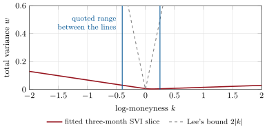
The bound 2 is reached only if the underlying has no finite moment beyond the first; a lognormal, with all moments, has slope zero. An SVI fit whose wing slope $b(1\pm\rho)$ exceeds 2 has an arbitrage in its extrapolation, whatever it does inside the quoted range, and a fit constrained to $b(1+|\rho|)\le2$ cannot produce one there (Figure 8.1).

A good fit slice by slice does not make a good surface: two slices fitted independently can cross, which is a calendar arbitrage (chapter 7). The surface version solves that by tying the slices together through the at-the-money total variance.

Definition 8.3 (Surface SVI)

Surface SVI (SSVI) writes the whole surface as a function of log-moneyness and the at-the-money total variance $\theta_T$ of each expiry,

$$w(k,\theta_T)=\frac{\theta_T}2\Bigl(1+\rho\varphi(\theta_T)k+\sqrt{\bigl(\varphi(\theta_T)k+\rho\bigr)^2+1-\rho^2}\Bigr),$$

with one correlation-like parameter $\rho$ and a curvature function $\varphi$, commonly the power law $\varphi(\theta)=\eta\theta^{-\gamma}$.

Theorem 8.4 (No-arbitrage conditions for SSVI)

An SSVI surface with $\theta_T$ non-decreasing in $T$ is free of calendar arbitrage if $0\le\partial_\theta(\theta\varphi(\theta))\le\frac{1}{\rho^2}\bigl(1+\sqrt{1-\rho^2}\bigr)\varphi(\theta)$; for the power law this holds whenever $0<\gamma<1$. It is free of butterfly arbitrage if, for every $\theta$, $\theta\varphi(\theta)(1+|\rho|)<4$ and $\theta\varphi(\theta)^2(1+|\rho|)\le4$.

The theorem and its proof are in Gatheral and Jacquier; the first butterfly condition is also necessary. With the power law and $\gamma=\tfrac12$, the at-the-money skew in volatility is $\rho\eta/(2\sqrt T)$: the $T^{-1/2}$ decay of equity skews that chapter 12 will revisit.

Example 8.5 (One surface, five numbers)

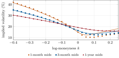
Fitted to the tutorial’s five expiries (one month to two years), SSVI returns $\rho=-0.560$, $\eta=1.095$, $\gamma=0.478$ and satisfies both conditions. It misses the mids by 0.09 volatility points at one year, 0.76 at three months and 2.0 at one month (Figure 8.2): the market’s short smiles are more skewed than one $\rho$ can describe. Desks use SSVI as the arbitrage-free backbone and add slice-by-slice corrections where the quotes demand them.

8.3 Splines and non-parametric fits

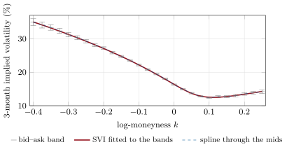
The alternative to a formula is a flexible curve: a cubic spline in $k$ through the quotes, or a smoothing spline that trades closeness to the quotes against roughness. A spline through the mids reproduces them exactly, noise included; on the tutorial’s three-month slice it strays up to 0.17 volatility points from the smile the quotes were drawn from, twice as far as the SVI fit (0.08), and its second derivative, which is the density, inherits the noise (Figure 8.3). A smoothing spline removes most of that at the cost of a parameter (the smoothing weight) that has no market meaning; and neither kind of spline says anything about the wings beyond the last strike, nor guarantees the absence of arbitrage without explicit constraints. Splines are used where no formula fits (a smile with two humps around a binary event) and as a check on a parametric fit.

8.4 Fitting to bid and ask

A mid is not a price at which anyone trades. What the market says is that the fair value of each option lies between its bid and its ask, and any smile inside every band is consistent with it.

Method 8.6 (Fitting SVI to a band of quotes)

For one expiry with quotes $w^{\mathrm{bid}}_j\le w^{\mathrm{ask}}_j$ at $k_j$:

1. Objective: the squared distance by which the model leaves each band, plus a small weight on the distance to the mid to break ties; weight each strike by the inverse square of its width, so that tight quotes count more.
2. Inner problem: for fixed $(m,\varsigma)$, with $y=(k-m)/\varsigma$, SVI is linear in $(a,\ b\rho\varsigma,\ b\varsigma)$; solve by weighted least squares and project on the domain $b(1+|\rho|)\le2$, $|\rho|<1$, $a\ge0$ (the quasi-explicit method).
3. Outer problem: minimise over the two remaining parameters $(m,\varsigma)$ by a derivative-free search from a few starting points.
4. Check the result: every fitted point inside its band (or report which are not), the wings within Lee’s bound, the density factor $g$ of chapter 7 non-negative on a fine grid.

On the tutorial’s three-month slice, 27 strikes with bands from 0.4 volatility points wide at the money to 2 points at the far left, the fit lands inside all 27 bands, with a largest distance to a mid of 0.18 points and parameters $a=0.0019$, $b=0.038$, $\rho=-0.63$, $m=0.059$, $\varsigma=0.066$.

8.5 Events, and business time against calendar time

A surface assumes that variance accrues smoothly with time. Two facts break that: known events, which add a lump of variance on one date, and weekends and holidays, on which almost none accrues.

Definition 8.7 (Event variance)

The event variance of a scheduled announcement (an earnings release, a central-bank decision, a trial result) is the variance of the log-return caused by the announcement itself. Between two expiries that bracket the event it is the excess of total variance over what the diffusive rate of the earlier expiry would accrue: $w_{\mathrm{event}}=w(T_2)-\bigl(w(T_1)/T_1\bigr)T_2$.

Example 8.8 (An earnings week)

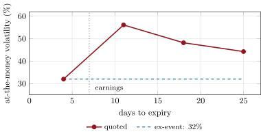
A share reports after the close on day 7. At-the-money volatilities are 32.0% for the expiry in 4 days, 56.1% in 11 days, 48.2% in 18 and 44.3% in 25. The event variance is $0.561^2\times11/365-0.32^2\times11/365=0.0064$: a standard deviation of 8.0% for the move on the announcement, an expected absolute move of $8.0\%\times\sqrt{2/\pi}=6.4\%$. Removing it, the 18-day expiry’s volatility is 32.0%: the whole term structure beyond the event is one diffusive volatility plus one jump (Figure 8.4).

Interpolating total variance linearly in calendar time between the 4-day and 11-day expiries would spread the jump over the week, and price a 7-day option (expiring before the announcement) at nearly 50% instead of 32%. Studies of individual equity options document the pattern: implied volatility rises into earnings and drops sharply after the release (Dubinsky and Johannes). Surfaces therefore carry a calendar of events, each with its own variance, fitted from the term structure and removed before any interpolation in time.

Definition 8.9 (Business time)

Business time is a clock that counts the variance-bearing time between two dates rather than calendar days: trading days count one, weekends and holidays a fraction (often zero), and event days one plus their event variance. Volatilities quoted on a 252-trading-day clock are in business time.

A one-week option at 20% on a 252-day clock (five trading days) is worth what a 20.34% volatility on the 365-day calendar clock gives over seven days. The difference shows up in theta: on the calendar clock a Friday-to-Monday roll costs two-sevenths of a week’s time value, on the business clock almost nothing, and the loss happens on the trading days instead. A desk that marks in calendar time and sees the market re-mark every Monday is using the wrong clock.

8.6 Tutorial: fitting a live slice

8.7 Build: the SVI fitter

8.8 Exercises

Exercise 8.1 ★

For the fitted three-month slice ($a=0.0019$, $b=0.038$, $\rho=-0.63$, $m=0.059$, $\varsigma=0.066$), give the total variance and the implied volatility at the money ($k=0$).

Solution

Solution of Exercise 8.1.

$w(0)=a+b\bigl(-\rho m+\sqrt{m^2+\varsigma^2}\bigr)=0.00670$; the implied volatility is $\sqrt{0.00670/(91/365)}=16.4\%$.

Exercise 8.2 ★

Give the left and right wing slopes of that slice, and the number of finite negative moments that the left slope implies by Lee’s formula.

Solution

Solution of Exercise 8.2.

Left $b(1-\rho)=0.062$, right $b(1+\rho)=0.014$. From $\tilde q=1/(2\beta_L)+\beta_L/8-1/2$ with $\beta_L=0.062$: $\tilde q=7.6$, so negative moments $\E S_T^{-q}$ are finite up to about $q=7.6$; far from the bound 2, which would mean no finite negative moment.

Exercise 8.3 ★

The expiry before an announcement (5 days) is at 30% and the one after (12 days) at 50%. Give the event variance, its standard deviation and the expected absolute move.

Solution

Solution of Exercise 8.3.

$0.5^2\times12/365-0.3^2\times12/365=0.00526$; standard deviation 7.3%; expected absolute move $7.3\%\times\sqrt{2/\pi}=5.8\%$.

Exercise 8.4 ★★

Why is interpolating total variance linearly in calendar time wrong between two expiries that bracket an earnings release? What does it do to an option expiring the day before the release?

Solution

Solution of Exercise 8.4.

The event adds variance at one date, not at a rate. Linear interpolation spreads it over the interval, so an option expiring the day before the release is charged part of the event’s variance it will never see: on the chapter’s numbers a 7-day option would be priced at 49.5% instead of 32%.

Exercise 8.5 ★★

With the fitted SSVI parameters, check both butterfly conditions at the one-month at-the-money total variance $\theta=0.00183$.

Solution

Solution of Exercise 8.5.

$\varphi=1.095\times0.00183^{-0.478}$; $\theta\varphi(1+|\rho|)=0.064<4$ and $\theta\varphi^2(1+|\rho|)=1.42\le4$: both hold.

Exercise 8.6 ★★

A one-week option is quoted at 25% on a 252-trading-day clock with five trading days left. Give the equivalent volatility on a 365-day calendar clock over seven days.

Solution

Solution of Exercise 8.6.

$\sigma_c=0.25\sqrt{(5/252)/(7/365)}=25.43\%$.

Exercise 8.7 ★★★

Coding. Fit SVI to the mids only, with equal weights, and compare the number of strikes inside their band and the wing slopes with the band fit.

Solution

Solution of Exercise 8.7.

On these quotes both fits lie inside all 27 bands and their wings are within $2\times10^{-4}$ of each other (0.0623 and 0.0140 against 0.0621 and 0.0142). The band fit matters when quotes are wide or lopsided, and in the wings, where mids are least reliable.

Exercise 8.8 ★★★

Find the flaw. “The spline passes through every mid, so its fitting error is zero; SVI misses the mids by up to 0.18 points. The spline is the better surface.”

Solution

Solution of Exercise 8.8.

The mids are not the fair values: they carry noise of a fraction of the spread. Passing through them reproduces the noise (the spline is 0.17 points from the true smile at worst, SVI 0.08), puts it into the density and the Greeks, and says nothing about the wings. The right error measure is distance to the bid–ask band, which both satisfy, and stability of the surface from one refit to the next.

8.9 Problem: Earnings Week

Problem 8.1

Weekend problem — the move the options are pricing

A share reports earnings after the close on day 7. Its at-the-money implied volatilities, quoted to 0.1 point, are 32.0% (4 days), 56.1% (11 days), 48.2% (18 days) and 44.3% (25 days). A client asks how much the market thinks the share will move on the release, and what a straddle bought for the release costs.

Part I — Total variances.

1. Give the total variance of the 4-day and the 11-day expiries.
2. What total variance would the 11-day expiry have without the event?
3. Give the event variance.
4. Give its standard deviation and the expected absolute move of a normal jump with that deviation.
5. Why use the 4-day expiry, not the 25-day one, as the diffusive rate?

Part II — Consistency.

6. Remove the event from the 18-day expiry: what volatility remains?
7. Do the same for the 25-day expiry.
8. What would a remaining volatility well above 32% suggest?
9. What does the 11-day volatility become the day after the release, if nothing else changes?
10. Why does the 11-day straddle lose value overnight even if the share moves 6%?

Part III — The surface.

11. How should the surface interpolate between the 4-day and 11-day expiries?
12. Which expiries’ smiles should be steeper, and why?
13. How would you treat a weekend between the 4-day and 11-day expiries?
14. A 7-day option expires before the release: what volatility should it carry?
15. What happens to the fitted SVI parameters of the 11-day slice after the release?

Part IV — Judgement.

16. Is 6.4% the market’s forecast of the move?
17. How would you compare it with the share’s history of earnings moves?
18. What trade expresses the view that the move will be smaller than priced, and what is its risk?
19. State the named result: the standard deviation and the expected absolute size of the move priced by the options.
20. In one sentence: why must events be taken out before interpolating in time?

Solution

Solution of Problem 8.1.

1. $0.32^2\times4/365=0.001122$; $0.561^2\times11/365=0.009485$. 2. $0.32^2\times11/365=0.003086$. 3. $0.009485-0.003086=0.0064$. 4. 8.0% and 6.4%. 5. The 4-day expiry is the only one that ends before the release; later expiries all contain the event. 6. 32.0%. 7. 32.1%. 8. A second event before those expiries, or a market that expects higher diffusive volatility after the release. 9. About 32%: the event variance leaves the expiry’s total variance once the release is past. 10. The straddle was priced with the event’s variance; a 6% move is below the 8% standard deviation priced, and the volatility crush after the release takes the time value with it. 11. Linearly in total variance on a clock that puts the event’s variance on day 7 and the diffusive variance on the other trading days. 12. The expiries just after the release: a jump makes the smile more curved at short expiries, and more so the larger the event variance relative to the diffusive variance. 13. Give the weekend days little or no variance in business time. 14. The diffusive 32%. 15. The slice’s level falls sharply and the curvature that the jump added near the money goes; the refit’s parameters jump accordingly, which is why parameter changes on event dates are expected, not alarms. 16. No: it is the move priced under the pricing measure, including a premium for bearing the event risk. 17. Compare the implied expected absolute move with the average absolute move on the share’s past releases, measured the same way (close before to close after). 18. Sell the 11-day straddle and buy the 4-day or a later expiry to hedge the diffusive volatility; the risk is a move larger than priced, a loss of gamma on the release day. 19. A standard deviation of 8.0% and an expected absolute move of 6.4%. 20. Because an event adds variance on one date, and interpolation in time would spread it over expiries that end before it.

8.10 Interview questions

Interview question 8.1 ★ researcher, trader

Write SVI and say what each parameter does to the smile.

Solution

Solution of Interview question 8.1.

$w(k)=a+b(\rho(k-m)+\sqrt{(k-m)^2+\varsigma^2})$: $a$ raises the whole smile, $b$ opens the angle between the wings, $\rho$ rotates it (skew), $m$ shifts it left or right, $\varsigma$ rounds the vertex.

What the interviewer is looking for: the formula and the geometric role of each parameter.

Interview question 8.2 ★ trader

From the at-the-money volatilities of the expiries before and after an earnings release, how do you get the implied move?

Solution

Solution of Interview question 8.2.

Compute total variances; the event variance is the later expiry’s total variance minus the earlier expiry’s variance rate times the later expiry’s time; its square root is the standard deviation of the move, and $\sqrt{2/\pi}$ times it the expected absolute move.

What the interviewer is looking for: working in total variance, not volatility.

Interview question 8.3 ★★ researcher

Why can total implied variance not grow faster than $2|k|$ in the wings?

Solution

Solution of Interview question 8.3.

Lee’s moment formula: the slope of total variance in the wing is $2-4(\sqrt{p^2+p}-p)$, where $p$ counts the finite moments of the underlying; it is at most 2, attained when no moment beyond the first is finite. A steeper wing would give call prices that violate arbitrage bounds at extreme strikes.

What the interviewer is looking for: the bound, and its link to moments.

Interview question 8.4 ★★ researcher, developer

You fit SVI every second on 20 expiries. How do you make the fit fast and stable, and how do you fit to bid and ask rather than to mids?

Solution

Solution of Interview question 8.4.

Reduce the dimension: for fixed $(m,\varsigma)$ SVI is linear in three parameters, solved by least squares; search the remaining two from yesterday’s (or the last second’s) values; impose Lee’s bound and the admissible domain; minimise distance outside the bands with weights by width; check arbitrage after each fit and fall back to the previous surface if a check fails.

What the interviewer is looking for: dimension reduction, warm starts, bands, checks.

Interview question 8.5 ★★ trader, risk

Your desk marks theta in calendar time. What happens every Monday morning, and what should change?

Solution

Solution of Interview question 8.5.

Friday’s marks include two days of calendar theta that the market does not charge; on Monday the options are re-marked higher than the model expects, and the desk books an apparent vega gain that is the weekend theta coming back. Move to business time, with weekend weights.

What the interviewer is looking for: the clock as a modelling choice.

Interview question 8.6 ★★★ researcher

When would you choose SSVI over independent SVI slices, and what do you give up?

Solution

Solution of Interview question 8.6.

SSVI when the surface must be free of arbitrage by construction and stable (risk systems, exotics pricing, sparse or illiquid expiries), and to extrapolate in expiry; independent slices when each expiry must match its quotes closely (market making). SSVI gives up the fit of short, steep smiles, since one $\rho$ and one curvature law span all expiries.

What the interviewer is looking for: guarantees against flexibility.