Derivatives and Volatility · Derivatives

7Implied Volatility and Its Surface

Before October 1987 the implied volatilities of S&P 500 index options were roughly the same at every strike: a flat line, as the Black–Scholes model says they should be. After the crash, in which the index fell by a fifth within two days, low strikes began to trade at higher volatilities than high strikes, and they have done so ever since. On a quiet day now, a three-month put 10% below the market costs 20 volatility while the call 10% above costs 14; a put 20% below costs 27, and prices a fall that the at-the-money volatility of 16 would call a one-in-three-hundred event as a one-in-fifty event. The model has not changed; the prices have. Since then the model has been used as a unit of measure: every option is quoted by the volatility that the formula needs to reproduce its price, and the table of those numbers across strikes and expiries is what an options desk looks at, fits, trades and risk-manages. This chapter describes that table, the rules it must obey, and what it says about the distribution the market is pricing.

7.1 The surface as the market’s price list

Implied volatility is defined in One Quant Book 1, chapter 25, with the skew across strikes and the term structure across expiries. Put together they form a surface, and two changes of coordinates make it comparable across expiries and underlyings.

Definition 7.1 (Volatility surface, log-moneyness, total implied variance)

The volatility surface of an underlying is the function $(K,T)\mapsto\sigma_{\mathrm{imp}}(K,T)$ that gives, for every strike and expiry, the implied volatility of the European option, computed with Black’s formula on the forward $F_{0,T}$ of that expiry. Its natural coordinates are the log-moneyness $k=\ln(K/F_{0,T})$ , which measures a strike against the forward of its own expiry, and the total implied variance $w(k,T)=\sigma_{\mathrm{imp}}^2T$ , the variance of the log-return to expiry that the price implies.

In these coordinates Black’s formula depends on $(k,w)$ only, up to the factor $P(0,T)F_{0,T}$ : $C/(PF)=\Phi(-k/\sqrt w+\sqrt w/2)-e^k\Phi(-k/\sqrt w-\sqrt w/2)$ . A surface is then a family of smiles $k\mapsto w(k,T)$ , one per expiry, and the static no-arbitrage conditions of the next sections become conditions on $w$ .

**Figure 7.1.** The chapter’s equity-index surface: four smiles of one surface. Short expiries are steep and low at the money; long expiries are flatter and higher. The 90–110 skew is 10.8 volatility points at one month, 6.3 at three months, 3.3 at one year and 2.5 at two. Illustrative parameters, in line with the shapes described in the text.

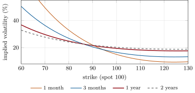
The surface is also the desk’s price list. A quote for any European option on the underlying, however unusual its strike or expiry, is read from it; a structured product priced by a model calibrated to it inherits its skew; and the risk of the whole book is measured against moves of it.

7.2 Smile phenomenology by asset class

The shapes differ by market, and the differences have reasons.

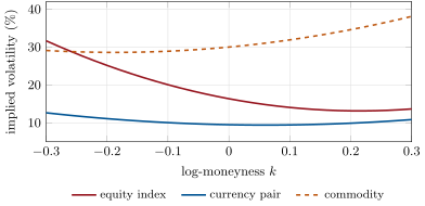
Equity indices: a steep negative skew, steeper for short expiries and decaying roughly like a power of the expiry (chapter 12), with the at-the-money level low in calm markets and the term structure upward-sloping. Investors buy index puts as insurance, crashes happen downward, and volatility rises when prices fall.
Single stocks: skewed the same way but less, with more curvature: studies of individual equity options find their risk-neutral distributions far less negatively skewed than the index’s. The index skew adds the tendency of stocks to fall together, the correlation skew of chapter 17.
Currencies: nearly symmetric smiles around the at-the-money level, tilted by the risk reversal towards the currency that is feared to fall (One Quant Book 2, chapter 19).
Commodities: often skewed upwards. A supply shock raises the price and the volatility together, and most commodities show higher volatility after price rises, the reverse of the equity pattern; crude oil is the documented exception (Figure 7.2).
Interest rates: quoted in normal volatility (One Quant Book 2, chapter 13), with smiles modelled by SABR (chapter 11) and a cube of expiries, tenors and strikes built in One Quant Book 6, chapter 5.

**Figure 7.2.** Three-month smiles by asset class, as functions of log-moneyness: an equity index skewed down, a currency pair nearly symmetric, a commodity skewed up. Illustrative shapes.

7.3 Sticky strike, sticky delta and what the desk assumes

A surface is a snapshot. When the spot moves, something must be assumed about how the surface moves with it, and the assumption changes the hedge.

Definition 7.2 (Sticky strike and sticky delta)

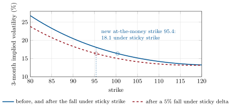
Under sticky strike the implied volatility of each strike and expiry stays fixed when the spot moves: the smile, drawn against strike, does not move. Under sticky delta (also sticky moneyness) the implied volatility of each moneyness $K/F$ stays fixed: the smile moves with the forward, and the at-the-money volatility does not change.

The two rules are regimes rather than laws: studies of index volatilities find periods in which each describes the market better, and a third in which the at-the-money volatility moves more than either predicts (Derman). They matter for three reasons. They give different P&L for the same move: after a 5% fall of the index, the three-month put struck at 100 is worth 6.00 under sticky strike and 5.78 under sticky delta, from 3.08 before (Figure 7.3). They give different deltas.

Proposition 7.3 (Smile-adjusted delta)

If the implied volatility of a fixed strike moves with the spot as $\partial\sigma_{\mathrm{imp}}/\partial S$ , the option’s total delta is $\Delta_{\mathrm{BS}}+\mathcal V\,\partial\sigma_{\mathrm{imp}}/\partial S$ . Under sticky strike the correction is zero; under sticky delta, with the smile a function of $k=\ln(K/F)$ , $\partial\sigma_{\mathrm{imp}}/\partial S=-\sigma_{\mathrm{imp}}'(k)/S$ , which is positive for a negative skew.

Proof. Differentiate $V=C_{\mathrm{BS}}(S,\sigma_{\mathrm{imp}}(K,T;S))$ in $S$ ; with $\sigma_{\mathrm{imp}}=\Sigma(\ln K-\ln F)$ and $F$ proportional to $S$ , $\partial\sigma_{\mathrm{imp}}/\partial S=-\Sigma'(k)/S$ . ∎

For the three-month call struck at 100 on the chapter’s surface, the Black–Scholes delta is 0.533 and the sticky-delta delta 0.593: a desk that assumes one regime and lives in the other is under- or over-hedged by six shares per hundred options. And they give different exotic prices, because a model of the surface’s dynamics (local volatility, chapter 9; stochastic volatility, chapter 10) implies one regime or the other; chapter 11 measures the difference.

**Figure 7.3.** The three-month smile before and after a 5% fall of the index. Under sticky strike the curve stays where it was and the new at-the-money strike (95.4) reads 18.1 volatility on it; under sticky delta the curve shifts left with the forward and the at-the-money volatility stays at 16.4. Round markers: at-the-money points. Data: the tutorial.

7.4 Static no-arbitrage conditions

Not every table of numbers is a surface. Chapter 1 listed the model-free inequalities on the prices of one expiry; across expiries one more family is needed.

Definition 7.4 (Static arbitrage, butterfly and calendar arbitrage)

A static arbitrage in a set of option quotes is a portfolio of the options, the forward and bonds, bought once and held to the expiries, that costs nothing and pays a non-negative amount in every state, positive in some. A butterfly arbitrage is one inside an expiry: call prices that are not convex in the strike, so that a butterfly has a negative price. A calendar arbitrage is one across expiries: a longer-dated option cheaper than the shorter-dated one at the same forward-moneyness.

The absence of call-spread, butterfly and calendar arbitrage is sufficient to exclude all static arbitrage from a surface of quotes on one underlier (Carr and Madan). In total variance the conditions are simple.

Proposition 7.5 (Static arbitrage in total variance)

With deterministic rates and dividends proportional to the share: (i) there is no calendar arbitrage if and only if $w(k,T)$ is non-decreasing in $T$ for every $k$ ; (ii) a smile $k\mapsto w(k)$ is free of butterfly arbitrage if and only if the call prices it implies are convex in the strike, which holds when

g(k)=\Bigl(1-\frac{kw'}{2w}\Bigr)^2-\frac{w'^2}{4}\Bigl(\frac1w+\frac14\Bigr)+\frac{w^{\prime\prime}}{2}\ \ge0

for every $k$ , together with call prices that tend to zero for large strikes.

Partial proof. (i) At fixed $k$ , the normalised call $C/(PF)$ is an increasing function of $w$ alone; a calendar spread at fixed forward-moneyness is a call on a martingale at two dates, whose value increases with the date by Jensen’s inequality, hence $w$ must increase. (ii) The second strike derivative of the call equals the density of the next section, and computing it through $w(k)$ gives $g(k)$ times a positive factor $\varphi(d_2)/\sqrt w$ ; the full statement is proved by Gatheral and Jacquier. ∎

A single bad quote is enough to break a surface. On the chapter’s surface, raising the three-month volatility at $k=-0.1$ by three points makes $g$ negative at six points of that smile, down to $-2.06$ : the butterfly centred there would have a negative price. Lowering the six-month at-the-money quote by seven points makes $w$ fall between three and six months: a calendar arbitrage. The surface builder of this chapter checks both before any model is calibrated to the surface (chapter 8).

7.5 The risk-neutral density

Definition 7.6 (Risk-neutral density and the Breeden–Litzenberger formula)

The risk-neutral density of $S_T$ is the density $q_T(s)$ of the underlying at $T$ under the risk-neutral measure (One Quant Book 4, chapter 5); it is the continuous version of the state prices of chapter 1, divided by the discount factor. The Breeden–Litzenberger formula reads it off call prices:

q_T(K)=\frac{1}{P(0,T)}\,\frac{\partial^2C(K,T)}{\partial K^2}.

Derivation. The call is the discounted expected payoff,

C(K,T)=P(0,T)\int_K^\infty(s-K)\,q_T(s)\,ds .

Differentiating once in $K$ gives $-P(0,T)\int_K^\infty q_T(s)\,ds$ , minus the discounted digital, and once more gives the formula. ∎

The first derivative is already a statement about the skew: the price of a digital call is $-\partial C/\partial K=P(0,T)\Phi(d_2)-\mathcal V\,\partial\sigma_{\mathrm{imp}}/\partial K$ , the Black–Scholes digital plus a skew correction. With a negative skew the correction is positive: the three-month at-the-money digital call on the chapter’s surface is worth 0.558, against 0.498 without the skew.

Example 7.7 (The crash premium)

On the chapter’s surface the three-month forward is 100.37 and the at-the-money volatility 16.36%. With a flat surface at that level the risk-neutral probability that the index ends below 80 is 0.31%; with the skew, whose 80 strike is at 26.8 volatility, it is 1.89%, six times more (Figure 7.4). The 80 put costs 0.006 on the flat surface and 0.219 on the skewed one.

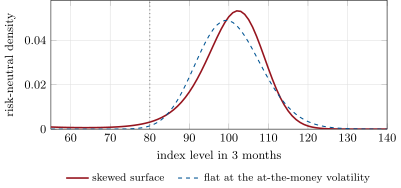
**Figure 7.4.** Risk-neutral densities of the index in three months from Breeden–Litzenberger applied to call prices: with the chapter’s skew (solid) and with a flat surface at the same at-the-money volatility (dashed). The skew moves probability into the left tail and makes the density’s peak sit above the forward; the probability below 80 (dotted) rises from 0.31% to 1.89%. Data: the tutorial.

The density is a price, not a forecast. It includes what investors pay for protection, and its left tail is fatter than the real-world frequency of crashes if insurance commands a premium, as chapter 14 measures on variance. What it is exactly is the portfolio of options that pays one unit if the index ends in a small interval around $s$ : the Arrow–Debreu security of chapter 1 made continuous, and replicable from the strip of listed options.

7.6 Tutorial: building and checking a surface

Goal. Build a surface from quotes in total variance, check it for static arbitrage, break it with a bad quote, and read the risk-neutral density off it. End state: Figures 7.1 and 7.4 and the numbers of Example 7.7.

The checks: the density factor $g$ on every slice, and $w$ across slices.

def density_factor(w: float, w1: float, w2: float, k: float) -> float:
    """g(k): the risk-neutral density of k equals g(k) / sqrt(2 pi w) exp(-d2^2 / 2)."""
    return (1 - k * w1 / (2 * w)) ** 2 - w1 * w1 / 4 * (1 / w + 0.25) + w2 / 2


def arbitrage_report(s: Surface, k_grid=None) -> dict[str, list]:
    """Calendar violations (i, k) where w falls between expiries i-1 and i, and butterfly violations
    (i, k, g) where the density factor is negative."""
    k_grid = np.linspace(min(s.ks), max(s.ks), 81) if k_grid is None else k_grid
    cal, fly = [], []
    for i in range(len(s.expiries)):
        for k in k_grid:
            w, w1, w2 = s._slice(i, float(k))
            if i > 0 and w < s._slice(i - 1, float(k))[0] - 1e-12:
                cal.append((i, float(k)))
            g = density_factor(w, w1, w2, float(k))
            if g < -1e-10:
                fly.append((i, float(k), g))
    return {"calendar": cal, "butterfly": fly}

Listing 7.1. Butterfly and calendar checks in total variance. code/firm/volsurface/firm_volsurface.py

The crash premium: the probability below a level is the strike derivative of the put, so the skew enters through the derivative of the volatility.

def crash_probability(level: float = 80.0, days: int = 91) -> dict[str, float]:
    """Risk-neutral probability that the index ends below `level`: minus the strike derivative of the
    put, discounted back, with and without the skew."""
    t = days / 365.0
    f, df = forward(t), math.exp(-RATE * t)
    h = 0.01

    def put(k, flat):
        vol = smile_vol(0.0, t) if flat else smile_vol(math.log(k / f), t)
        return black(f, k, t, df, vol, "P")
    skew = (put(level + h, False) - put(level - h, False)) / (2 * h) / df
    flat = (put(level + h, True) - put(level - h, True)) / (2 * h) / df
    atm = smile_vol(0.0, t)
    d2 = (math.log(f / level) - 0.5 * atm * atm * t) / (atm * math.sqrt(t))
    return {"skewed": skew, "flat": flat, "flat_formula": ncdf(-d2), "ratio": skew / flat,
            "vol_at_80": smile_vol(math.log(level / f), t), "atm": atm}

Listing 7.2. Risk-neutral probability of a fall, with and without the skew. code/derivatives/07-implied-volatility-and-its-surface/python/dv_surface.py

Run dv_surface.check(index_surface()) (no violation), check(index_surface((1, -0.1, 0.03))) (six), crash_probability() and fig_surface.py.

What to change next. Interpolate each smile linearly in $k$ instead of by a cubic spline and count the butterfly violations the kinks create; then build the surface on a strike grid rather than a moneyness grid and look for calendar violations near ex-dividend dates.

7.7 Build: the volatility surface

Purpose. The miniature firm’s single object for implied volatility: fits (chapter 8), models (chapters 9–13) and the pricing library (chapter 28) read from it, and nothing downstream of it may see an arbitrage.

Interface. Surface(asof, expiries, ks, w, forwards) with implied_vol(strike, expiry), total_variance(k, t), forward(t); from_vols(asof, expiries, forwards, ks, vols); arbitrage_report(surface); density_factor; risk_neutral_density(strikes, calls, df).

Rules. Interpolate total variance: a not-a-knot cubic spline in $k$ within an expiry (a natural spline bends a convex smile the wrong way at its ends), linear in $t$ at fixed $k$ between expiries, flat volatility before the first and after the last; extrapolate linearly in $k$ and report the wings as a risk (chapter 8).

Acceptance tests. code/firm/volsurface/tests/: the surface returns its input volatilities at the nodes; a surface built from a flat volatility has a density factor of one at $k=0$ and no violation; a bumped quote creates butterfly violations and a lowered long expiry a calendar violation; Breeden–Litzenberger recovers the lognormal density.

Stretch. Replace the node grid by the SVI slices of chapter 8, and add a sticky-delta mode that re-centres the surface on a new forward.

Sources and further reading

E. Derman, The Volatility Smile, lecture notes, Columbia University (2008), lecture 1; and “Regimes of volatility”, Risk (April 1999).
M. Rubinstein, “Implied binomial trees”, Journal of Finance 49 (1994) 771–818.
D. T. Breeden and R. H. Litzenberger, “Prices of state-contingent claims implicit in option prices”, Journal of Business 51 (1978) 621–651.
P. Carr and D. B. Madan, “A note on sufficient conditions for no arbitrage”, Finance Research Letters 2 (2005) 125–130.
G. Bakshi, N. Kapadia and D. Madan, “Stock return characteristics, skew laws, and the differential pricing of individual equity options”, Review of Financial Studies 16 (2003) 101–143.
Y.-F. Chen and X. Mu, “Asymmetric volatility in commodity markets”, Journal of Commodity Markets 22 (2021).
J. Gatheral, The Volatility Surface, Wiley, 2006.

7.8 Exercises

Exercise 7.1 ★

The three-month forward is 100.37. Give the log-moneyness of the strike 90 and its total variance at 20.47 volatility.

Solution

Solution of Exercise 7.1.

$k=\ln(90/100.37)=-0.1091$ ; $w=0.2047^2\times91/365=0.0104$ .

Exercise 7.2 ★

On the chapter’s surface the three-month 90 and 110 strikes are at 20.47 and 14.19 volatility. Give the 90–110 skew and explain why the same skew in strike terms would be smaller at one year.

Solution

Solution of Exercise 7.2.

$20.47-14.19=6.27$ volatility points. At one year the same strikes are closer to the money in standard deviations ( $\ln(K/F)/\sqrt T$ is halved), and the skew per unit of $k$ is itself smaller, decaying roughly like $T^{-1/2}$ : the one-year 90–110 skew is 3.3 points.

Exercise 7.3 ★

At the same forward-moneyness $k=0$ , the three-month option is quoted at 20% and the six-month at 13%. Is there a calendar arbitrage? What would you trade?

Solution

Solution of Exercise 7.3.

$w$ is $0.2^2\times0.25=0.0100$ at three months and $0.13^2\times0.5=0.0085$ at six: total variance falls, a calendar arbitrage. Sell the three-month straddle (or call) and buy the six-month one at the same forward-moneyness: the long-dated option is worth at least the short-dated one at the first expiry.

Exercise 7.4 ★★

Price the three-month at-the-money digital call on the chapter’s surface with and without the skew correction, given a vega of 19.77 and a volatility slope $\partial\sigma/\partial K$ of $-0.0031$ per unit of strike.

Solution

Solution of Exercise 7.4.

Without the skew: $P\Phi(d_2)=0.4980$ . The correction is $-\mathcal V\,\partial\sigma/\partial K =19.77\times0.0031=0.0604$ (per unit of volatility): 0.5584 with the skew.

Exercise 7.5 ★★

Give the three-month call’s delta at the 100 strike under sticky strike and under sticky delta, and say how many shares per 100 calls the choice changes.

Solution

Solution of Exercise 7.5.

Sticky strike: the Black–Scholes delta, 0.533. Sticky delta: $0.533+19.77\times0.00306=0.593$ . Six shares per 100 calls.

Exercise 7.6 ★★

Why is an equity index’s skew steeper than the skews of its members?

Solution

Solution of Exercise 7.6.

An index’s risk-neutral distribution adds the members’ tendency to fall together: in a crash correlations rise, so the index’s left tail is fatter than any member’s relative to its own volatility. Individual risk-neutral distributions are far less negatively skewed than the index’s; the gap is the correlation skew of chapter 17.

Exercise 7.7 ★★★

Coding. With index_surface and check, add a quote error of $+3$ points at three months and $k=-0.1$ : how many butterfly violations, and how negative does $g$ get? Then find the smallest downward error on the six-month at-the-money quote that creates a calendar violation.

Solution

Solution of Exercise 7.7.

Six butterfly violations, the worst at $g=-2.06$ at $k=-0.1$ . A downward error of 6 points on the six-month at-the-money quote leaves $w$ increasing; 6.5 points (the first half-point step that does) creates one calendar violation, 7 points one, 8 points three.

Exercise 7.8 ★★★

Find the flaw. “The three-month 80 put is at 27 volatility against 16 at the money: the market expects the index to be twice as volatile if it falls to 80.”

Solution

Solution of Exercise 7.8.

Implied volatility at a strike is a price, not the volatility expected if the index reaches that strike. The 80 put’s 27 prices the probability and severity of a fall in one number, including a premium for insurance and for jumps, which no diffusion volatility at 80 describes. What the market would expect conditional on a fall is the local volatility of chapter 9 or the model’s dynamics, not the implied volatility at that strike.

7.9 Problem: The Crash Premium

Problem 7.1

Weekend problem — what the skew says about a 20% fall

A pension fund asks what the index options say about a fall of more than 20% over the next three months, and what protection against it costs. Use the chapter’s surface: spot 100, rate 3%, dividend yield 1.5%, three months to expiry.

Part I — The inputs.

Give the three-month forward and discount factor.
Give the at-the-money volatility and the volatility at the 80 strike.
Give the log-moneyness of the 80 strike.
Price the 80 put on the skewed surface.
Price it on a flat surface at the at-the-money volatility.

Part II — Probabilities.

Give the risk-neutral probability of ending below 80 on the flat surface.
Give it on the skewed surface.
Why is it not $\Phi(-d_2)$ at the 80 strike’s own volatility?
How is the probability related to a digital put, and to a put spread?
Sketch where the skew moves probability, using the density.

Part III — Interpreting.

Is 1.89% a forecast of the frequency of such falls? Why not?
What else is in the price of the 80 put?
How would a 5% fall of the index change the 80 put under sticky strike and sticky delta?
Why did the skew appear after 1987?
Why might the skew be steeper at one month than at one year?

Part IV — Judgement.

What would you tell the fund about the cost of this protection?
What is the cheaper way to buy protection against a 20% fall, and what does it give up?
What should a risk system use for this probability: the flat or the skewed surface?
State the named result: the risk-neutral probability of a fall below 80 in three months on the flat and on the skewed surface, and their ratio.
In one sentence: what does the skew price?

Solution

Solution of Problem 7.1.

1. Forward 100.37; discount factor 0.99255. 2. 16.36% and 26.78%. 3. $\ln(80/100.37)=-0.2269$ . 4. 0.219. 5. 0.006. 6. 0.31%. 7. 1.89%. 8. The probability is minus the strike derivative of the put divided by the discount factor, and the put’s volatility changes with the strike: the skew adds $\mathcal V\, \partial\sigma/\partial K$ , which $\Phi(-d_2)$ at a fixed volatility ignores. 9. It is the forward value of a digital put struck at 80, and the limit of a put spread $(P(80+h)-P(80-h))/(2h)$ divided by the discount factor. 10. From the centre and the right tail into the left tail (and a little into the region just above the forward, where the peak rises). 11. No: it is a price, the probability under the measure that makes prices expectations, and includes the premium investors pay to avoid the fall. 12. The risk premium for crash insurance, the demand of hedgers, and the dealers’ cost of carrying the risk. 13. The put gains from the fall in both regimes; under sticky strike its volatility is unchanged at 26.8, under sticky delta it falls, since the put is now closer to the money (23.8 at the new moneyness): sticky strike gives the larger gain. 14. The crash showed that a fall of a fifth within two days was possible; buyers of protection and sellers who had lost repriced the left tail, and have kept doing so. 15. A fall is sudden: a jump or a burst of volatility is a larger share of the variance to a short expiry than to a long one, so short-dated skews are steeper (chapters 12–13). 16. That the market charges about six times the flat-volatility probability, and that the price is 0.22 per 100 of notional per quarter, about 0.9% a year if rolled. 17. A put spread (buy 80, sell 70) or a collar: cheaper, but the protection stops below 70, or the upside is given away. 18. The skewed surface, which is where the protection can actually be bought; the flat surface understates the tail by a factor of six. 19. 0.31% flat, 1.89% skewed: six times more. 20. The market’s price of the distribution’s left tail, above what one volatility can describe.

7.10 Interview questions

Interview question 7.1 ★ trader, researcher

Why do equity index options have a skew, and why did it appear only after 1987?

Solution

Solution of Interview question 7.1.

Investors buy index puts as insurance, crashes are downward and sudden, and volatility rises when prices fall; before 1987 the market priced near-lognormal tails, and the crash showed that a fall of a fifth in a day or two was possible. Sellers of puts have charged for it since.

What the interviewer is looking for: demand for insurance, jumps, the leverage effect, and the historical break.

Interview question 7.2 ★ researcher

How do you get the risk-neutral density from option prices?

Solution

Solution of Interview question 7.2.

Breeden–Litzenberger: $q(K)=\partial^2C/\partial K^2/P(0,T)$ . In practice fit an arbitrage-free smile first (raw quotes are too noisy to differentiate twice), then differentiate the smooth call prices; check that the density integrates to one and reprices the forward.

What the interviewer is looking for: the formula and the need to smooth first.

Interview question 7.3 ★★ trader

The index falls 5%. Under sticky strike and under sticky delta, what happens to the at-the-money volatility and to your delta?

Solution

Solution of Interview question 7.3.

Sticky strike: each strike keeps its volatility, so the new at-the-money volatility is read higher up the skew (18.1 from 16.4 in the chapter) and delta is the Black–Scholes delta. Sticky delta: the smile moves with the forward, at-the-money volatility is unchanged, and delta adds vega times the slope, higher for a negative skew.

What the interviewer is looking for: both the level change and the hedge change.

Interview question 7.4 ★★ researcher, developer

Give the static no-arbitrage conditions on an implied-volatility surface, and how you check them.

Solution

Solution of Interview question 7.4.

Calls decreasing in strike and with slope above $-P(0,T)$ ; convex in strike (butterflies non-negative), equivalently $g(k)\ge0$ in total variance; total variance non-decreasing in expiry at fixed forward-moneyness. Check each slice on a fine grid of $k$ and each pair of consecutive slices; with bid and ask, check at executable prices.

What the interviewer is looking for: the three conditions and their total-variance form.

Interview question 7.5 ★★ risk

A risk report computes the probability of a 20% fall from the at-the-money volatility. What is wrong, and by how much can it be off?

Solution

Solution of Interview question 7.5.

It uses a lognormal tail, ignoring the skew. The probability is the strike derivative of the put, which includes the skew term; on a typical index surface the error at 20% below is a factor of five or more (six in the chapter).

What the interviewer is looking for: the skew in the derivative, and the size of the error.

Interview question 7.6 ★★★ developer, researcher

How would you interpolate a surface between quoted strikes and expiries without creating arbitrage?

Solution

Solution of Interview question 7.6.

Work in total variance and log-moneyness; within an expiry use a smooth parametrisation or a spline in $k$ that respects $g\ge0$ (SVI, chapter 8), with care at the ends; between expiries interpolate $w$ linearly in time at fixed $k$ , which preserves calendar monotonicity; handle dividends and events in the time coordinate; check the result.

What the interviewer is looking for: total variance, monotone interpolation in time, and a check.

Terms defined in this chapter

See all 2333 terms in the glossary