Derivatives and Volatility · Derivatives

15Barriers and Digitals

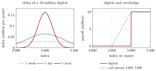
A desk has sold a digital option that pays 10 million if the index closes above 5 000. One minute before the close the index is at 4 999.9. The option is worth 4.9 million, and a move of one index point in either direction changes that by 1.25 million. To hedge it, the desk would need an index position equivalent to 6.25 billion, bought or sold in the last minute of trading and reversed if the index ticks back. No desk does that. The digital’s discontinuity makes it unhedgeable at the strike near expiry. The same discontinuity sits at the level of every barrier option, which the market trades in large size in currencies and inside structured products. This chapter prices digitals and barriers and explains how desks hedge what cannot be delta-hedged, with an overhedge, with static portfolios of vanillas, and with a shifted barrier for discrete monitoring. It ends with the risk that none of these remove, a price that jumps over the barrier.

15.1 Digitals and their hedge

Definition 15.1 (Digital option)

A digital option (binary option) pays a fixed amount if the underlying ends above (call) or below (put) the strike, and nothing otherwise. Under Black–Scholes a cash digital call paying 1 is worth $e^{-rT}\Phi(d_2)$ .

A digital is the limit of call spreads, $\bigl(C(K-\varepsilon)-C(K)\bigr)/\varepsilon$ as $\varepsilon\to0$ , so its price is minus the strike derivative of the call price. With a smile the call’s volatility depends on the strike, and differentiating gives

D(K)=-\frac{\partial C}{\partial K}=D_{\mathrm{BS}}(K,\sigma(K))-\mathcal V(K)\,\frac{\partial\sigma}{\partial K}.

With a downside skew $\partial\sigma/\partial K<0$ , so the digital call is worth more than its Black–Scholes price at the strike’s volatility. The skew term is often the larger part of the difference between desks’ quotes.

Example 15.2 (A three-month digital on chapter 9’s surface)

Scale chapter 9’s surface to an index at 5 000. A three-month at-the-money digital call on 10 million is worth 4.84 million with Black–Scholes at the at-the-money volatility of 16.4%. With the smile it is worth 5.77 million: the vega term adds 0.93 million, almost a fifth of the price.

Near expiry the digital’s delta, $e^{-rT}\varphi(d_2)/(S\sigma\sqrt T)$ per unit paid, grows like $1/\sqrt T$ at the strike and vanishes away from it (Figure 15.1, left). Its gamma changes sign at the strike. A desk short a digital near the strike is either short or long a huge convexity, depending on which side of the strike the index sits, and it cannot trade fast enough to follow. The practical answer is to replace the digital by a call spread.

Definition 15.3 (Call-spread overhedge)

The call-spread overhedge prices and hedges a sold digital call as the call spread that dominates it: $N/\varepsilon$ calls struck at $K-\varepsilon$ less as many struck at $K$ . The spread pays at least the digital everywhere, and the difference in price, the overhedge, is charged to the buyer.

The width $\varepsilon$ trades price against risk. A narrow spread is cheap but keeps most of the digital’s convexity: its delta can reach $N/\varepsilon$ per index point. A wide spread is easy to hedge but charges the client for a payoff he did not buy. A desk sets the width from the largest loss it will accept per point of the settlement price, the point at which the spread’s slope becomes the risk. On the example, widths of 50, 100, 200 and 400 index points cost 0.25, 0.48, 0.89 and 1.56 million over the digital’s 5.77 million.

Figure 15.1. Left: the delta of a 10-million digital struck at 5 000 (20% volatility) as expiry approaches; one minute before the close it reaches 1.25 million per point, off this scale. Right: the digital’s payoff and the call spread that overhedges it; the extra payoff between 4 800 and 5 000 is what the overhedge charges for. Data: the chapter’s code.

15.2 Barriers by reflection

A barrier option (One Quant Book 2, chapter 19) switches on or off when the underlying touches a level $H$ . With continuous monitoring and Black–Scholes dynamics, all eight single barriers have closed forms, and all follow from the reflection principle (One Quant Book 4, chapter 2).

Proposition 15.4 (The down-and-out call by images)

For $K\ge H$ , carry $b=r-q$ and $\nu=b-\frac12\sigma^2$ , the down-and-out call is

C_{\mathrm{DO}}(S)=C_{\mathrm{BS}}(S,K)-\Bigl(\frac HS\Bigr)^{2\nu/\sigma^2}C_{\mathrm{BS}}\Bigl(\frac{H^2}S,K\Bigr).

Proof. The function $u(S,t)=(H/S)^{2\nu/\sigma^2}C_{\mathrm{BS}}(H^2/S,K,t)$ solves the Black–Scholes equation, which can be checked by substitution. It equals $C_{\mathrm{BS}}(H,K)$ on $S=H$ , and its terminal payoff vanishes for $S>H$ when $K\ge H$ , because $H^2/S<H\le K$ there. The difference is therefore the solution that pays the call above the barrier and zero on it. In the driftless log-price this is the method of images: the path density killed at $H$ is the free density less its reflection in $H$ . ∎

The other seven, with their in-out parity $V_{\mathrm{in}}+V_{\mathrm{out}}=V_{\mathrm{vanilla}}$ and rebates, are combinations of four terms of this kind. The build implements all eight and tests parity for every case.

Definition 15.5 (Barrier rebate)

A barrier rebate is a fixed amount paid to the holder of a knock-out option when the barrier is hit, or to the holder of a knock-in option at expiry if it never knocked in.

Definition 15.6 (One-touch option)

A one-touch option pays a fixed amount if the underlying touches the barrier before expiry, either at the hit or at expiry.

Definition 15.7 (No-touch option)

A no-touch option pays a fixed amount at expiry if the underlying never touches the barrier. A one-touch paid at expiry and a no-touch on the same barrier add up to a zero-coupon bond.

Definition 15.8 (Double-barrier option)

A double-barrier option has a lower and an upper barrier, and knocks in or out when either is touched. The double no-touch, which pays if neither is touched, is its simplest form.

Touch options are digitals on the path’s extremes. The probability of touching a lower barrier $H<S$ by $T$ is $\Phi\bigl((x-\nu T)/\sigma\sqrt T\bigr)+e^{2\nu x/\sigma^2}\Phi\bigl((x+\nu T)/\sigma\sqrt T\bigr)$ , with $x=\ln(H/S)$ . A double barrier has no finite formula. Its killed density is a sine series in the log-price, whose terms decay like $e^{-k^2\pi^2\sigma^2T/(2a^2)}$ for a corridor of log-width $a$ , so a few dozen terms suffice.

Example 15.9 (A barrier sheet)

Spot and strike 100, one year, $r=3\%$ , $q=1\%$ , volatility 20%. The call is worth 8.83. With a knock-out at 90 it is worth 7.23, and the down-and-in 1.60, which adds up. A rebate of 2 paid at the hit raises the knock-out to 8.41, since the one-touch at 90 paid at the hit is worth 0.592 (0.581 paid at expiry). The no-touch at 90 is worth 0.390, the up-and-out call with barrier 130 is worth 3.10, and the double no-touch between 85 and 115 is worth 0.141 (Figure 15.3, left).

15.3 Static hedging

A barrier’s delta is discontinuous at the barrier, as the digital’s is at its strike. The alternative to dynamic hedging is a portfolio of vanillas that matches the barrier’s value on the barrier and its payoff at expiry, so that it can be unwound at no cost when the barrier is hit.

Definition 15.10 (Static hedging)

Static hedging replicates an exotic option with a portfolio of vanilla options fixed at inception, traded again only at events such as a barrier hit or expiry, rather than rebalanced continuously.

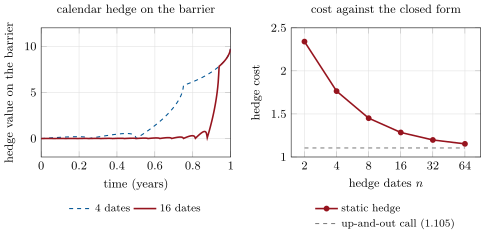
Carr, Ellis and Gupta’s put–call symmetry gives the simplest static hedges. With zero carry and no smile, a call struck at $K$ is worth, on the barrier $H$ , exactly as much as $K/H$ puts struck at $H^2/K$ , at every time. A down-and-in call is therefore hedged by holding $K/H$ puts at $H^2/K$ . If the barrier is hit, the desk swaps them for the call at no cost. If it is not, the puts, whose strike is below the barrier, expire worthless, as the knock-in does. With strike 100, barrier 90, one year and 20% volatility, the hedge is 1.11 puts struck at 81, worth 1.498, the closed-form price exactly.

The symmetry needs a symmetric smile, and an index smile is not symmetric. Suppose the barrier is hit with six months left and chapter 9’s six-month smile keeps its shape in moneyness. The 1.11 puts struck at 81 are then worth 2.08 and the call struck at 100 only 0.83. The downside skew prices the puts, which sit below the barrier, at higher volatilities than the call above it. A static hedge built from the symmetry would have cost far more than the option. Skew breaks every model-free static hedge of this kind. Derman, Ergener and Kani’s calendar hedge instead holds options of several expiries chosen, under a model, so that the portfolio is worth zero on the barrier at a set of dates.

Example 15.11 (A calendar hedge of an up-and-out call)

Strike 100, barrier 120, one year, 20%, zero carry: the up-and-out call is worth 1.105. The terminal payoff is a call at 100 less a call at 120 less 20 digitals at 120. Working back over $n$ equally spaced dates, the desk adds calls struck at 120 of each expiry in the amounts that zero the portfolio on the barrier at each date. With 4 dates the hedge costs 1.77 and is worth up to 5.4 on the barrier between dates, over the first nine months. With 16 dates it costs 1.28 and is worth at most 0.16. With 64 it costs 1.15 (Figure 15.2). The error halves each time the dates double. The last interval before expiry is the hardest, because there the payoff on the barrier jumps from 20 to 0.

**Figure 15.2.** A static hedge of an up-and-out call (strike 100, barrier 120, one year, 20%) from calls of several expiries. Left: the hedge’s value on the barrier through time: zero at the dates it is built on, and large in the last interval, where the payoff jumps. Right: its cost converges to the option’s price as the dates multiply. Data: the tutorial.

15.4 Discrete monitoring and the barrier shift

Most barrier contracts outside currencies are monitored at discrete dates: daily closes or fixings. A discretely monitored knock-out survives paths that dipped through the barrier between observations, so it is worth more than the continuous formula says. Broadie, Glasserman and Kou showed that the continuous formula becomes accurate again if the barrier is moved away from the spot.

Definition 15.12 (Barrier shift)

The barrier shift prices an option monitored every $\Delta t$ with the continuous formula at the barrier $H\,e^{\pm\beta\sigma\sqrt{\Delta t}}$ , moved away from the spot, with $\beta\approx0.5826$ .

The constant is $-\zeta(\frac12)/\sqrt{2\pi}$ , the expected overshoot of a Gaussian random walk over a level, in units of its step. The build keeps it in one named constant.

Example 15.13 (How good is the shift)

The knock-out call of Example 15.9 (barrier 90) is worth 7.23 with continuous monitoring. With daily monitoring, a Monte Carlo of 200 000 paths gives 7.48 (standard error 0.03), and the shifted formula 7.45. With weekly monitoring they give 7.62 and 7.68, with monthly 8.01 and 8.04, and with four dates 8.33 and 8.38 (Figure 15.3, right). For an up-and-out call with barrier 120, where the payoff is large at the barrier, the shift is good daily (1.26 against 1.28) and poor quarterly (2.19 against 2.50). The correction is an expansion in $\sqrt{\Delta t}$ and fails when the barrier is within a few steps of the spot or the payoff at the barrier is large.

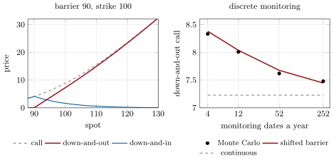
**Figure 15.3.** Left: a call, its down-and-out and its down-and-in by spot (one year, 20%); they add up. Right: the down-and-out call monitored 4, 12, 52 and 252 times a year: Monte Carlo against the continuous formula and the formula at the shifted barrier. Data: the tutorial.

The flat-volatility formula has a larger error than monitoring when the smile is steep. Under chapter 9’s local volatility, the same knock-out (zero rates, one year, daily monitoring) is worth 6.15 by simulation, against 6.51 from the shifted Black–Scholes formula at the at-the-money volatility of 19.2%. Local volatility is higher at low spots, so the barrier is hit more often. How far the smile moves such prices depends on the smile’s dynamics as well as its level, local volatility against stochastic volatility (chapters 9 and 10). Chapter 20 prices currency barriers with the market’s own correction, built from the option’s vanna and volga.

15.5 Gap risk at the barrier

Every hedge in this chapter assumes the price passes through the barrier: the static hedge is unwound at the barrier, the dynamic hedge trades near it, the stop-loss order is filled at it. A price that jumps over the barrier defeats all three.

Definition 15.14 (Gap risk)

Gap risk is the risk that a price moves discontinuously across a level at which a position’s value or hedge changes, a barrier, a strike near expiry, or a stop, so that the hedge planned at that level is executed at a worse price or not at all.

The reverse knock-out, whose payoff is large at the barrier, carries it in the purest form.

Example 15.15 (A gap through a reverse barrier)

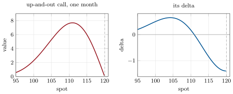
An up-and-out call, strike 100, barrier 120, has one month left, and the spot is 119. It is worth 1.38 and its delta is $-1.37$ : a rise brings the barrier closer and destroys the payoff (Figure 15.4). The seller hedges by selling 1.37 shares. If the spot moves to 119.5, the hedged position’s P&L is $+0.005$ . If it gaps to 125, the option dies, and the seller gains its 1.38, but the short shares lose $1.37\times6=8.19$ : a net loss of 6.81, five times the premium.

**Figure 15.4.** A reverse knock-out near its barrier: strike 100, barrier 120 (dashed), one month left, 20%. Its value peaks well before the barrier and its delta turns strongly negative; a hedger short the option is short the underlying there, and loses on any gap through the barrier. Data: the chapter’s code.

Gaps are not only a matter of weekends and earnings. On 15 January 2015 the Swiss National Bank discontinued its minimum exchange rate of 1.20 Swiss francs per euro. The ECB’s euro reference rate for the franc was 1.2010 on the 14th and 1.0280 on the 15th, a fall of 14.4% between two fixings, and 1.0128 on the 16th. A barrier anywhere in that range was crossed in a single move, and a hedge planned at the barrier could only be executed wherever the market next traded. A floor that a central bank defends looks like the safest barrier in the market, and when it fails, it fails by a gap. Desks price the risk with jump models (chapter 13) and hold reserves for it (chapter 27).

15.6 Tutorial: barriers and digitals

Goal. Price a digital with and without a smile and its call-spread overhedge; price barriers in closed form, under discrete monitoring and under local volatility; build two static hedges; measure the gap. End state: the four figures and the numbers of the weekend problem.

A digital under a smile is minus the strike derivative of the call:

def digital_smile(s: float, k: float, t: float, r: float, q: float, vol_of_k, h: float | None = None) -> float:
    """Digital call under a smile: minus the strike derivative of the call price, which is the flat-volatility
    digital minus vega times the smile's slope in strike."""
    h = 1e-4 * k if h is None else h
    return -(bs(s, k + h, t, r, q, vol_of_k(k + h), "C") - bs(s, k - h, t, r, q, vol_of_k(k - h), "C")) / (2 * h)

Listing 15.1. The smile-consistent digital. code/firm/barrier/firm_barrier.py

The barrier shift and its check. The shifted barrier, and a Monte Carlo of discretely monitored barriers with exact lognormal steps:

def bgk_shift(h: float, s: float, vol: float, dt: float) -> float:
    """The continuous barrier that prices a barrier monitored every dt: moved away from the spot by
    exp(beta sigma sqrt(dt))."""
    return h * math.exp((1 if h > s else -1) * BGK_BETA * vol * math.sqrt(dt))


def mc_barrier(s: float, k: float, h: float, t: float, r: float, q: float, vol: float, kind: str, right: str,
               steps: int, n_paths: int = 200_000, seed: int = 15) -> tuple[float, float]:
    """Monte Carlo of a barrier monitored at `steps` equally spaced dates (exact lognormal steps, antithetic).
    Returns (price, standard error)."""
    rng = np.random.default_rng(seed)
    dt = t / steps
    z = rng.standard_normal((n_paths // 2, steps))
    z = np.vstack([z, -z])
    logs = math.log(s) + np.cumsum((r - q - 0.5 * vol * vol) * dt + vol * math.sqrt(dt) * z, axis=1)
    paths = np.exp(logs)
    hit = (paths.min(axis=1) <= h) if kind.startswith("down") else (paths.max(axis=1) >= h)
    alive = ~hit if kind.endswith("out") else hit
    st = paths[:, -1]
    pay = np.maximum(st - k, 0.0) if right == "C" else np.maximum(k - st, 0.0)
    x = math.exp(-r * t) * pay * alive
    return float(x.mean()), float(x.std() / math.sqrt(len(x)))

Listing 15.2. Barrier shift and discrete-monitoring Monte Carlo. code/firm/barrier/firm_barrier.py

A double no-touch by its sine series:

def double_no_touch(s: float, lo: float, hi: float, t: float, r: float, q: float, vol: float,
                    terms: int = 200) -> float:
    """Pays 1 at expiry if the price stays strictly inside (lo, hi): the killed transition density of the log price
    expanded in sines, p(y) = (2/a) sum_k sin(k pi y0 / a) sin(k pi y / a) e^(c (y - y0) - (mu^2 / (2 sigma^2) +
    k^2 pi^2 sigma^2 / (2 a^2)) T), integrated over y in closed form."""
    mu = r - q - 0.5 * vol * vol
    a = math.log(hi / lo)
    y0 = math.log(s / lo)
    c = mu / (vol * vol)
    total = 0.0
    for k in range(1, terms + 1):
        bk = k * math.pi / a
        integral = bk * (1 - (-1) ** k * math.exp(c * a)) / (c * c + bk * bk)
        total += (2 / a) * math.sin(bk * y0) * integral * math.exp(
            -c * y0 - (mu * mu / (2 * vol * vol) + 0.5 * bk * bk * vol * vol) * t)
    return math.exp(-r * t) * total

Listing 15.3. Double no-touch. code/firm/barrier/firm_barrier.py

Run dv_barrier.digital_prices(), overhedge(200), monitoring(), local_vol_doc(), calendar_example(), reverse_barrier() and fig_barrier.py.

What to change next. Price the digital as a call spread centred on the strike and compare its risk with the overhedge; replace the calls at the barrier in the calendar hedge by puts; move the up-and-out barrier to 110 and re-run the gap.

15.7 Build: barriers and digitals

Purpose. The miniature firm’s barrier and digital pricer: closed forms with rebates, touches, double no-touch, the discrete-monitoring shift, and a static-hedge builder; the engine that chapter 18’s autocallables and chapter 20’s currency barriers call.

Interface. digital, digital_delta, digital_smile(s, k, t, r, q, vol_of_k); call_spread(…, width, notional, below); barrier(s, k, h, t, r, q, vol, kind, right, rebate) with kind in down-out, down-in, up-out, up-in; hit_probability, one_touch(…, at_hit), no_touch, double_no_touch; bgk_shift, BGK_BETA; mc_barrier; symmetry_down_in_call; calendar_hedge, calendar_hedge_on_barrier.

Rules. In and out always add up to the vanilla (tested for all eight cases); discrete monitoring is priced with the shift or by simulation, never with the continuous formula; a digital is always priced with the smile’s slope; a digital sold is booked at its overhedge.

Acceptance tests. code/firm/barrier/tests/: in-out parity for every kind, right and strike; a distant barrier gives the vanilla; the shifted formula matches a daily Monte Carlo; touch identities, and the double no-touch against its single-barrier limit and a simulation; the smile digital reduces to the flat one without skew, and call spreads bracket the digital; the symmetry hedge prices the down-and-in exactly, and the calendar hedge converges.

Stretch. Barriers under local and stochastic volatility by finite differences (chapter 22); window barriers; the vanna–volga correction of chapter 20.

Sources and further reading

M. Broadie, P. Glasserman and S. Kou, “A continuity correction for discrete barrier options”, Mathematical Finance 7(4) (1997) 325–349.
E. Derman, D. Ergener and I. Kani, “Static options replication”, Journal of Derivatives 2(4) (1995) 78–95.
P. Carr, K. Ellis and V. Gupta, “Static hedging of exotic options”, Journal of Finance 53(3) (1998) 1165–1190.
Swiss National Bank, press release, 15 January 2015; European Central Bank, euro foreign exchange reference rates.

15.8 Exercises

Exercise 15.1 ★

Show that a cash digital call and a cash digital put on the same strike and expiry add up to a zero-coupon bond. What does that imply for their deltas?

Solution

Solution of Exercise 15.1.

Exactly one of the two pays 1 at expiry, whatever happens, so together they pay 1 for sure: a zero-coupon bond, $e^{-rT}$ . Their deltas therefore add up to zero: the digital put’s delta is minus the call’s.

Exercise 15.2 ★

Why does a downside skew make a digital call more expensive than its Black–Scholes price at the strike’s volatility?

Solution

Solution of Exercise 15.2.

The digital is $-\partial C/\partial K$ . With a downside skew the call’s volatility falls as the strike rises, so the call loses value with the strike faster than at a constant volatility, and $-\partial C/\partial K$ gains the term $-\mathcal V\,\partial\sigma/\partial K>0$ . In terms of probabilities: the skewed density has a fat left tail and, to keep the forward fixed, more mass just above the forward, so the probability of finishing above an at-the-money strike is higher than the flat model’s.

Exercise 15.3 ★

A knock-out call and its knock-in are priced at 7.23 and 1.70 while the vanilla is 8.83. What is wrong?

Solution

Solution of Exercise 15.3.

In-out parity is violated: $7.23+1.70=8.93\ne8.83$ . With zero rebates the two must add up to the vanilla; the knock-in should be 1.60, or one of the prices uses different inputs (barrier, monitoring or volatility).

Exercise 15.4 ★★

With zero carry, check the symmetry hedge numerically: price 1.11 puts struck at 81 and the down-and-in call with barrier 90 at 20% volatility. Why do the puts expire worthless whenever the barrier is not hit?

Solution

Solution of Exercise 15.4.

$K/H=1.11$ puts struck at $H^2/K=81$ are worth 1.498, and the down-and-in call is worth 1.498. If the barrier is never hit the index stays above 90 and ends above 90, hence above the puts’ strike of 81: the puts expire worthless, like the knock-in.

Exercise 15.5 ★★

A barrier is monitored daily at 20% volatility. By how much does the shift move a barrier at 90? At 120?

Solution

Solution of Exercise 15.5.

The factor is $e^{0.5826\times0.2\times\sqrt{1/252}}=e^{0.0073}$ : the barrier at 90 moves down to 89.34 and the barrier at 120 up to 120.88, away from the spot in both cases.

Exercise 15.6 ★★

Explain why the up-and-out call of Example 15.15 has a negative delta near the barrier, and why its value peaks below the barrier.

Solution

Solution of Exercise 15.6.

As the spot rises towards 120 the call’s intrinsic value grows, but so does the probability of touching the barrier and losing everything; near the barrier the second effect dominates, so the value falls with the spot and the delta is negative. The value peaks where the two effects balance, well below the barrier (near 111 with one month left, where it is worth 7.68).

Exercise 15.7 ★★★

Coding. Re-run the discrete-monitoring comparison for a down-and-out put with barrier 90. Does the shift work as well as for the call?

Solution

Solution of Exercise 15.7.

Continuous 0.162. Daily: Monte Carlo 0.205, shifted 0.207; weekly 0.262 and 0.270; monthly 0.383 and 0.430; four dates 0.564 and 0.735. The shift works daily, and degrades faster than for the call as monitoring thins out, because the put’s payoff is large at the barrier ( $K-H=10$ ), where the expansion is least accurate.

Exercise 15.8 ★★★

Find the flaw. “Our barrier book is safe: every barrier has a stop-loss order resting at its level, so the hedge is executed exactly when the option knocks.”

Solution

Solution of Exercise 15.8.

A stop-loss order at the barrier is filled at the next available price. If the market gaps through the level (an announcement, a policy change, an overnight move), the fill is far beyond it and the hedge’s P&L is the gap times the position, as on 15 January 2015. Gap risk must be priced (jump models) and limited (by exposure at each barrier level), not assumed away.

15.9 Problem: The Digital at Expiry

Problem 15.1

Weekend problem — how wide a call spread

A client buys a three-month digital that pays 10 million if the index, now at 5 000, closes above 5 000 at expiry. The desk prices on chapter 9’s surface scaled to 5 000 and will book the digital at a call-spread overhedge. Its limit: a one-point error in the settlement price may not move the hedge by more than 50 000.

Part I — The digital.

Give the digital’s price with the at-the-money volatility and with the smile.
What is the vega term, and why is it positive?
One minute before expiry with the index at 4 999.9 and 20% volatility, give the digital’s delta per point and as index notional.
Why can that delta not be traded?
What is the digital’s gamma just below and just above the strike near expiry?

Part II — The overhedge.

Which call spread dominates the digital, and why is it the one the seller buys?
What width meets the desk’s limit?
Give the spread’s price and the overhedge charged to the client.
Give the overhedge for widths of 50, 100 and 400 points.
What does the client receive, relative to the digital, if the index settles at 4 900?

Part III — Barriers.

Give the one-year down-and-out call (strike 100, barrier 90, 20%, $r=3\%$ , $q=1\%$ ) and its knock-in.
Give it with daily monitoring by simulation and by the shift.
Give it under chapter 9’s local volatility and explain the difference from the flat price.
Give the double no-touch between 85 and 115.
Price the one-touch at 90 paid at the hit and at expiry, and explain the difference.

Part IV — Judgement.

Why is the overhedge fair to the client?
When would you use a centred call spread instead?
How would you hedge a reverse knock-out near its barrier?
State the named result: the call-spread width that caps the hedger’s loss at 50 000 per settlement point on the 10-million digital, and the overhedge it charges the client.
In one sentence: what do digitals and barriers share?

Solution

Solution of Problem 15.1.

1. 4.84 million at 16.4%; 5.77 million with the smile. 2. 0.93 million: $-\mathcal V\,\partial\sigma/\partial K$ , positive because the skew makes volatility fall with the strike. 3. 1.25 million per index point, equivalent to 6.25 billion of index. 4. It would have to be bought or sold within a minute and reversed at every tick through the strike: far beyond the market’s depth, and the hedge would lose the spread each time. 5. For the holder, large and positive just below the strike and large and negative just above it; the seller has the opposite. 6. Long calls at $K-\varepsilon$ , short calls at $K$ , in size $N/\varepsilon$ : it pays at least the digital everywhere, so the seller who holds it is never short at expiry. 7. $\varepsilon=10\,000\,000/50\,000=200$ points: the spread’s payoff changes by at most 50 000 per point. 8. 6.66 million; the overhedge is 0.89 million over the digital’s 5.77 million. 9. 0.25, 0.48 and 1.56 million. 10. 5 million, half the digital’s notional, instead of nothing: the overhedge pays for this region. 11. 7.23 and 1.60. 12. 7.48 (standard error 0.03) by simulation and 7.45 by the shift. 13. 6.15 against 6.51: local volatility rises as the index falls towards the barrier, so the barrier is hit more often than at a flat volatility. 14. 0.141. 15. 0.592 at the hit, 0.581 at expiry: paying at the hit saves the discounting from the hit to expiry. 16. The client buys a payoff that dominates the digital; the extra price pays for the extra payoff between 4 800 and 5 000 and for a hedge the desk can actually run. 17. When the desk can accept some pin risk in exchange for a price close to the digital’s, for instance when it can offset it against other positions struck nearby; a centred spread is cheaper but can leave the seller short at expiry. 18. Statically where possible (a calendar of options at the barrier), with a limit on the delta at the barrier and a reserve for gaps; dynamic hedging alone fails exactly when the barrier is crossed by a jump. 19. 200 index points: a call spread of 50 000 per point from 4 800 to 5 000, which charges the client an overhedge of 0.89 million on the 10-million digital (5.77 million). 20. A discontinuity, in the payoff or at the barrier, where the delta becomes unbounded and the hedge must be replaced by an overhedge, a static portfolio or a reserve.

15.10 Interview questions

Interview question 15.1 ★ trader

How do you price and hedge a digital option?

Solution

Solution of Interview question 15.1.

Price it as minus the strike derivative of the call price, which brings in the smile’s slope. Hedge it as a call spread: book the sold digital at the price of the dominating spread (the overhedge) and delta-hedge the spread, whose delta is bounded.

What the interviewer is looking for: the smile term and the overhedge.

Interview question 15.2 ★ researcher

Derive the price of a down-and-out call with the reflection principle.

Solution

Solution of Interview question 15.2.

The killed density of the log-price at a lower barrier is the free density minus its reflection in the barrier, weighted by the drift factor. Integrating the call payoff against it gives $C_{\mathrm{BS}}(S)-(H/S)^{2\nu/\sigma^2}C_{\mathrm{BS}}(H^2/S)$ for $K\ge H$ ; check that it solves the Black–Scholes equation, is zero on the barrier and has the right payoff.

What the interviewer is looking for: the image, and the boundary check.

Interview question 15.3 ★★ trader, researcher

Why does the skew matter for a digital, and in which direction?

Solution

Solution of Interview question 15.3.

A digital is $-\partial C/\partial K$ , so it depends on the smile’s slope at the strike: $-\mathcal V\partial\sigma/\partial K$ . With a downside skew that term is positive for a digital call (worth more than its Black–Scholes price) and negative for a digital put.

What the interviewer is looking for: the derivative and the sign.

Interview question 15.4 ★★ developer

Your Monte Carlo prices a daily-monitored knock-out above the closed form. Is that a bug?

Solution

Solution of Interview question 15.4.

No: a daily-monitored knock-out misses crossings between observations, so it is worth more than the continuous formula. Compare with the formula at the barrier shifted by $e^{\beta\sigma\sqrt{\Delta t}}$ away from the spot; if the two agree within the simulation error, the Monte Carlo is right.

What the interviewer is looking for: discrete against continuous monitoring, and the shift.

Interview question 15.5 ★★ risk

What is gap risk on a barrier book, and how would you measure and limit it?

Solution

Solution of Interview question 15.5.

The loss if the underlying jumps through a barrier or strike where the position’s value or hedge changes abruptly. Measure it by scenario: the book’s P&L for jumps of several sizes across each barrier level, with hedges assumed filled at the post-jump price; limit the exposure concentrated at any one level, and price it with jump models or reserves.

What the interviewer is looking for: the scenario, concentration at levels, and pricing.

Interview question 15.6 ★★★ trader, researcher

Construct a static hedge for a down-and-in call. When does it fail?

Solution

Solution of Interview question 15.6.

With zero carry and a symmetric smile, hold $K/H$ puts struck at $H^2/K$ : on the barrier they are worth exactly the call, so at the hit swap them for it; if never hit they expire worthless. It fails with carry (the symmetry needs a driftless forward), with a skew (the puts below the barrier are priced at a higher volatility than the call above it), and with gaps through the barrier.

What the interviewer is looking for: the symmetry, and its three failure modes.

Terms defined in this chapter

See all 2333 terms in the glossary