Derivatives and Volatility · Derivatives

3Black–Scholes Three Ways

On 26 April 1973 the Chicago Board Options Exchange opened for business with calls on 16 stocks and traded 911 contracts. In the same spring the Journal of Political Economy printed a paper by Fischer Black and Myron Scholes, with a companion by Robert Merton, that gave the price of such a call as a closed formula in five numbers: spot, strike, time, rate and volatility. The formula was right for a reason that surprised economists: the expected return of the share, the one number every investor argues about, is not among the five. This chapter derives the formula three times, because each derivation carries a different lesson: replication shows why the drift disappears and what a hedger actually does; the martingale route shows which expectation is being taken and how to generalise it; the binomial limit shows that nothing here needs continuous-time mathematics to be true, only to be convenient.

3.1 The model and the replication argument

Definition 3.1 (Black–Scholes model)

The Black–Scholes model is a market with a bank account growing at a constant rate $r$ and a share that pays a continuous dividend yield $q$ and follows a geometric Brownian motion (One Quant Book 4, chapter 4) under the real-world measure,

dS_t=\mu S_t\,dt+\sigma S_t\,dW_t,

with constant $\mu$ and $\sigma>0$ . Trading is continuous and frictionless, short sales are allowed, and cash can be borrowed and lent at $r$ .

Let $V(t,S)$ be the value of a European claim paying $g(S_T)$ , assumed smooth in $(t,S)$ . Hold the claim and sell $\Delta$ shares. The short position pays the dividend $qS\,dt$ to the lender of the share. By Itô’s formula (One Quant Book 4, chapter 3) the position $\Pi=V-\Delta S$ changes by

d\Pi=\Bigl(\partial_tV+\tfrac12\sigma^2S^2\partial_{SS}V-q\Delta S\Bigr)dt +\bigl(\partial_SV-\Delta\bigr)\,dS .

Choosing $\Delta=\partial_SV$ removes the only random term. A portfolio with no risk must earn the riskless rate, or borrowing to buy it (or selling it to lend) would be an arbitrage: $d\Pi=r\Pi\,dt=r(V-S\partial_SV)\,dt$ . Equating the two expressions of $d\Pi$ gives the pricing equation.

Definition 3.2 (Black–Scholes equation)

The Black–Scholes equation is the parabolic partial differential equation

\partial_tV+(r-q)S\,\partial_SV+\tfrac12\sigma^2S^2\,\partial_{SS}V-rV=0, \qquad V(T,S)=g(S),

satisfied by the value of any European claim on the share in the Black–Scholes model.

The drift $\mu$ multiplied $dS$ , and $dS$ was hedged away: it cancelled with the position in shares. What survived is the variance term $\tfrac12\sigma^2S^2 \partial_{SS}V$ , which no position in shares can cancel because it comes from the curvature of $V$ , and the financing of the hedge at $r-q$ . The equation is linear, so the value of a portfolio of claims is the sum of the values, and it is the same for every investor whatever their view of $\mu$ .

Remark 3.3 (What the hedger does)

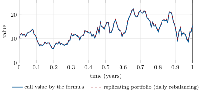
Selling the claim and holding $\Delta=\partial_SV$ shares financed at $r$ is a self-financing strategy (chapter 1) whose value tracks $V$ exactly in the model. Figure 3.1 runs it once, rebalanced daily along a path simulated with a drift of 12% a year: the portfolio follows the option, and the gap at expiry, 0.39 on a premium of 10.45, is the cost of hedging daily instead of continuously, the subject of chapter 4.

$Replication along one path. A one-year at-the-money call (r=5\%, =20\%) is replicated by holding shares and borrowing, rebalanced 252 times; the share, simulated with a drift of 12%, ends at 115.46. The two curves are indistinguishable at this scale; the final gap is 0.39. Data: the tutorial.$

Figure 3.1. Replication along one path. A one-year at-the-money call (

r=5\%

\sigma=20\%

) is replicated by holding

\Delta

shares and borrowing, rebalanced 252 times; the share, simulated with a drift of 12%, ends at 115.46. The two curves are indistinguishable at this scale; the final gap is 0.39. Data: the tutorial.

3.2 The pricing equation

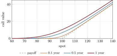
The Black–Scholes equation is a backward heat equation in disguise. With $x=\ln S$ and time to expiry $\tau=T-t$ , and $V=e^{-r\tau}u$ , it becomes $\partial_\tau u=(r-q-\tfrac12\sigma^2)\partial_xu+\tfrac12\sigma^2\partial_{xx}u$ , a diffusion with constant coefficients. By the Feynman–Kac formula (One Quant Book 4, chapter 4) its solution is an expectation:

V(t,S)=e^{-r(T-t)}\,\E\bigl[g(S_T)\mid S_t=S\bigr],\qquad dS_u=(r-q)S_u\,du+\sigma S_u\,d\widetilde W_u .\tag{3.1}

The expectation is taken for a share that grows at $r-q$ , not at $\mu$ : the equation knows nothing of $\mu$ , so neither does its solution. This is where the phrase “risk-neutral” comes from: prices are expectations as if investors required no premium for risk. It is a statement about prices, which is how chapter 1 read it, not about investors.

The call struck at 100 as a solution of the pricing equation, at three times to expiry (r=5\%, =20\%). Going back in time the payoff’s kink at the strike is smoothed out by diffusion and the curve is lifted by the interest on the strike. Data: the chapter’s code. — **Figure 3.2.** The call struck at 100 as a solution of the pricing equation, at three times to expiry ( $r=5\%$ , $\sigma=20\%$ ). Going back in time the payoff’s kink at the strike is smoothed out by diffusion and the curve is lifted by the interest on the strike. Data: the chapter’s code.

3.3 The martingale route

Chapter 1 priced a claim as a discounted expectation under a measure in which discounted traded prices are martingales. In the Black–Scholes model Girsanov’s theorem (One Quant Book 4, chapter 5) gives it explicitly: under the risk-neutral measure $\mathbb Q$ the process $W^{\mathbb Q}_t=W_t+\frac{\mu-r+q} {\sigma}t$ is a Brownian motion and

S_T=S_0\exp\Bigl(\bigl(r-q-\tfrac12\sigma^2\bigr)T+\sigma W^{\mathbb Q}_T\Bigr),

so that $e^{-(r-q)t}S_t$ is a $\mathbb Q$ -martingale: the dividend-adjusted share, discounted at $r$ , is a fair game. The price of the call is

C=e^{-rT}\E^{\mathbb Q}\bigl[(S_T-K)\mathbf 1_{S_T>K}\bigr] =e^{-rT}\E^{\mathbb Q}\bigl[S_T\mathbf 1_{S_T>K}\bigr]-Ke^{-rT}\,\mathbb Q(S_T>K).

The second term is a normal probability. The first needs one more idea: change the numeraire to the share (with its dividends reinvested). Under the share measure $\mathbb Q^S$ , with density $S_Te^{qT}/(S_0e^{rT})$ , the first expectation becomes $S_0e^{(r-q)T}\,\mathbb Q^S(S_T>K)$ , and under $\mathbb Q^S$ the log-share has drift $r-q+\tfrac12\sigma^2$ instead of $r-q-\tfrac12\sigma^2$ .

Theorem 3.4 (Black–Scholes formula)

In the Black–Scholes model the European call and put are worth

C=Se^{-qT}\Phi(d_1)-Ke^{-rT}\Phi(d_2),\qquad P=Ke^{-rT}\Phi(-d_2)-Se^{-qT}\Phi(-d_1),

d_{1,2}=\frac{\ln(S/K)+(r-q)T}{\sigma\sqrt T}\pm\tfrac12\sigma\sqrt T,

the Black–Scholes formula. Here $\Phi(d_2)=\mathbb Q(S_T>K)$ is the risk-neutral probability of exercise and $\Phi(d_1)=\mathbb Q^S(S_T>K)$ the same probability under the share measure, and $e^{-qT}\Phi(d_1)=\partial_SC$ is the hedge ratio.

Proof. $\ln S_T$ is normal with variance $\sigma^2T$ under both measures and with means differing by $\sigma^2T$ ; $\mathbb Q(S_T>K)=\Phi(d_2)$ and $\mathbb Q^S(S_T>K)= \Phi(d_1)$ follow by standardising. The put follows by put–call parity. The identity $\partial_SC=e^{-qT}\Phi(d_1)$ uses $S e^{-qT}\varphi(d_1)=Ke^{-rT} \varphi(d_2)$ , which cancels the terms from differentiating $d_1$ and $d_2$ . ∎

Example 3.5 (The desk’s reference call)

$S=K=100$ , $T=1$ , $r=5\%$ , $q=0$ , $\sigma=20\%$ : $d_1=0.35$ , $d_2=0.15$ , $\Phi(d_1)=0.6368$ , $\Phi(d_2)=0.5596$ , $C=10.4506$ , $P=5.5735$ . The risk-neutral probability of exercise is 0.56; with a real-world drift of 12% the probability that the call ends in the money is 0.69, and it plays no role in the price.

Proposition 3.6 (At-the-money approximation)

At the forward, $K=F=Se^{(r-q)T}$ , the call and the put are both worth $e^{-rT}F\bigl(2\Phi(\tfrac12\sigma\sqrt T)-1\bigr)\approx0.4\,e^{-rT}F\sigma\sqrt T$ .

Proof. With $K=F$ , $d_{1,2}=\pm\tfrac12\sigma\sqrt T$ and $C=e^{-rT}F(\Phi(d_1)-\Phi(-d_1))$ ; expand $\Phi$ at 0 with slope $\varphi(0)=1/\sqrt{2\pi}\approx0.3989$ . ∎

3.4 The binomial limit

The Cox–Ross–Rubinstein tree of chapter 2 needs no stochastic calculus and reaches the same number. With $n$ steps the tree call is the discounted expectation of $(S_T-K)^+$ under a binomial law of the number of up moves. As $n\to\infty$ with $u=e^{\sigma\sqrt{T/n}}$ , the tree’s probability of finishing above $K$ converges to $\Phi(d_2)$ , and the same probability computed with the weights $pu/R$ and $(1-p)d/R$ (the share measure on the tree) converges to $\Phi(d_1)$ : the two terms of the formula appear as limits of the two binomial sums of Proposition 2.4. For the reference call the 1 000-step tree gives 10.4486, 0.0020 below the formula, the error of order $1/n$ measured in chapter 2.

3.5 Black’s formula, and what each derivation teaches

Many underlyings are quoted as forwards or futures: commodity futures, bond futures, forward interest rates, FX forwards. Pricing on the forward removes the dividend yield, the borrow and the financing from the formula; they are all inside $F$ .

Definition 3.7 (Black model)

The Black model assumes that the forward (or futures) price $F_t$ of the underlying for delivery at $T$ is a driftless geometric Brownian motion under the $T$ -forward measure (One Quant Book 4, chapter 5): $dF_t=\sigma F_t\,dW^T_t$ . A European call with expiry $T$ is then worth

C=P(0,T)\bigl(F\Phi(d_1)-K\Phi(d_2)\bigr),\qquad d_{1,2}=\frac{\ln(F/K)}{\sigma\sqrt T}\pm\tfrac12\sigma\sqrt T .

The Black–Scholes formula is the special case $F=Se^{(r-q)T}$ , $P(0,T)=e^{-rT}$ . Black published the forward version in 1976 for commodity contracts; the futures options of One Quant Book 3, chapter 12, the caplets of One Quant Book 2, chapter 13, and the FX options of chapter 20 are all priced with it, and implied volatility is defined through it (One Quant Book 1, chapter 25). When the rate is stochastic, discounting with $P(0,T)$ and taking the expectation under the forward measure keeps the formula exact, provided the forward itself is lognormal.

Route	What it assumes	What it teaches
Replication	Itô’s formula, continuous hedging	why $\mu$ disappears; the hedge ratio; the equation generalises to any payoff and to numerical grids (chapter 22)
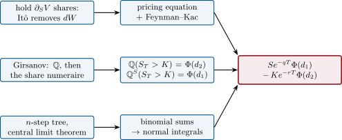
Martingale	a measure, a numeraire	which expectation is taken; the choice of numeraire simplifies payoffs; generalises to Monte Carlo (chapter 23) and to other dynamics (chapters 9–13)
Binomial limit	two-state steps	that the result is arbitrage, not calculus; American exercise (chapter 6)

**Figure 3.3.** Three routes to one formula: replication (top), the martingale expectation (middle), the limit of the binomial tree (bottom). Each needs a different piece of mathematics and each generalises to a different numerical method.

Method 3.8 (Implied volatility, robustly)

To invert Black’s formula at a price $c$ :

Check $P(0,T)(F-K)^+\le c<P(0,T)F$ (call); outside these bounds there is no volatility, and the quote or the forward is wrong.
Bracket: the price is increasing in $\sigma$ ; double an upper bound until it prices above $c$ .
Start from a closed-form guess on the time value and run Newton’s method with vega as derivative, falling back to bisection whenever a step leaves the bracket. Stop on relative price error ( $10^{-12}$ ).

Newton alone fails far from the money, where vega is tiny and a step overshoots; production libraries use rational approximations that converge in two iterations to machine precision (Jäckel).

3.6 Tutorial: one price, three ways

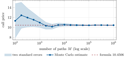
Goal. Implement Black’s formula and a robust implied-volatility solver, then price the reference call by the formula, a tree and Monte Carlo, and replicate it along a path. End state: Figures 3.1 and 3.4 and the numbers of the weekend problem.

The formula, on the forward, with a normal cdf accurate in the tails:

def black(fwd: float, strike: float, t: float, df: float, vol: float, right: str = "C") -> float:
    """Discounted Black price of a European call ("C") or put ("P") on a forward."""
    sign = 1.0 if right == "C" else -1.0
    if t <= 0.0 or vol <= 0.0:
        return df * max(sign * (fwd - strike), 0.0)
    s = vol * math.sqrt(t)
    d1 = math.log(fwd / strike) / s + 0.5 * s
    d2 = d1 - s
    return df * sign * (fwd * ncdf(sign * d1) - strike * ncdf(sign * d2))


def bs(spot: float, strike: float, t: float, r: float, q: float, vol: float, right: str = "C") -> float:
    """Black-Scholes price with a continuous dividend (or borrow) yield q."""
    return black(spot * math.exp((r - q) * t), strike, t, math.exp(-r * t), vol, right)

Listing 3.1. Black’s formula on a forward, and Black–Scholes on a spot. code/firm/bs/firm_bs.py

The solver of Method 3.8:

def implied_vol(price: float, fwd: float, strike: float, t: float, df: float, right: str = "C",
                tol: float = 1e-12, max_iter: int = 100) -> float:
    """Volatility at which black(...) equals price. Raises ValueError outside the arbitrage bounds."""
    sign = 1.0 if right == "C" else -1.0
    lo_p = df * max(sign * (fwd - strike), 0.0)
    hi_p = df * (fwd if right == "C" else strike)
    if not lo_p <= price < hi_p:
        raise ValueError(f"price {price} outside ({lo_p}, {hi_p}): no implied volatility")
    if price - lo_p < 1e-15 * df * max(fwd, strike):
        return 0.0
    # Brenner-Subrahmanyam / Corrado-Miller style guess on the time value, clipped to the bracket
    x = math.log(fwd / strike)
    c = price / df - 0.5 * sign * (fwd - strike)
    disc = max(c * c - (fwd - strike) ** 2 / math.pi, 0.0)
    guess = math.sqrt(2.0 * math.pi) / (fwd + strike) * (c + math.sqrt(disc)) / math.sqrt(t)
    lo, hi = 0.0, 1.0
    while black(fwd, strike, t, df, hi, right) < price:
        hi *= 2.0
        if hi > 100.0:
            raise ValueError("no volatility below 10000%")
    v = min(max(guess, 1e-4), hi) if guess > 0 and abs(x) < 1.0 else 0.5 * hi
    for _ in range(max_iter):
        f = black(fwd, strike, t, df, v, right) - price
        if abs(f) < tol * max(price, 1e-300) or hi - lo < 1e-15:
            return v
        if f > 0:
            hi = v
        else:
            lo = v
        s = v * math.sqrt(t)
        vega = df * fwd * npdf(x / s + 0.5 * s) * math.sqrt(t)
        step = v - f / vega if vega > 0 else -1.0
        v = step if lo < step < hi else 0.5 * (lo + hi)
    return v

Listing 3.2. Implied volatility: bounds, bracket, guess, safeguarded Newton. code/firm/bs/firm_bs.py

Monte Carlo: draw $S_T$ exactly from its lognormal law, average the discounted payoff, and report the standard error.

def mc_price(n_paths: int, seed: int = 2026, c: dict = CASE, antithetic: bool = False) -> tuple[float, float]:
    """Monte Carlo under Q: exact lognormal terminal draw. Returns (estimate, standard error)."""
    rng = np.random.default_rng(seed)
    z = rng.standard_normal(n_paths)
    if antithetic:
        z = np.concatenate([z, -z])
    s_t = c["spot"] * np.exp((c["r"] - c["q"] - 0.5 * c["vol"] ** 2) * c["t"] + c["vol"] * math.sqrt(c["t"]) * z)
    pay = math.exp(-c["r"] * c["t"]) * np.maximum(s_t - c["strike"], 0.0)
    if antithetic:
        pay = 0.5 * (pay[: n_paths] + pay[n_paths:])
    return float(pay.mean()), float(pay.std(ddof=1) / math.sqrt(len(pay)))

Listing 3.3. Monte Carlo under the risk-neutral measure, with its standard error. code/derivatives/03-black-scholes-three-ways/python/dv_blackscholes.py

Run dv_blackscholes.problem() and fig_blackscholes.py; the C++20 and Rust twins in code/firm/bs/ pass the same round-trip tests.

What to change next. Turn on antithetic variates and compare the standard error at equal work; rebalance the replicating portfolio weekly and hourly and compare the gap at expiry with the daily one.

Monte Carlo estimates of the reference call on the first M of one million draws. The band of two standard errors shrinks like 1/√ M: a hundred times more paths buy one more significant digit. Data: the tutorial. — **Figure 3.4.** Monte Carlo estimates of the reference call on the first $M$ of one million draws. The band of two standard errors shrinks like $1/\sqrt M$ : a hundred times more paths buy one more significant digit. Data: the tutorial.

3.7 Build: the Black–Scholes kernels

Purpose. The inner loop of the miniature firm: every surface fit, every Greek report, the risk engine of One Quant Book 6 and the pricing library of chapter 28 call these functions millions of times a day, so they exist in Python, C++20 and Rust with the same tests.

Interface. black(fwd, strike, t, df, vol, right); bs(spot, strike, t, r, q, vol, right); greeks(…) returning delta, gamma, vega, theta, rho, vanna and volga; implied_vol(price, fwd, strike, t, df, right). C++: firm::bs in cpp/firm_bs.hpp; Rust: crate firm_bs.

Rules. Price on the forward; $\Phi$ through the complementary error function so that deep out-of-the-money prices keep their relative accuracy; a price outside the arbitrage bounds raises, never returns a volatility.

Acceptance tests. code/firm/bs/tests/ and the C++ and Rust tests: the textbook value 10.450583572185579; parity with a dividend yield; each Greek against a central difference; implied-volatility round trips to a relative $10^{-11}$ over five decades of moneyness and maturities from a day to 30 years.

Stretch. Replace the solver by a rational-approximation method and measure iterations and time per inversion in the three languages.

Sources and further reading

F. Black and M. Scholes, “The pricing of options and corporate liabilities”, Journal of Political Economy 81 (1973) 637–654.
R. C. Merton, “Theory of rational option pricing”, Bell Journal of Economics and Management Science 4 (1973) 141–183.
F. Black, “The pricing of commodity contracts”, Journal of Financial Economics 3 (1976) 167–179.
P. Jäckel, “Let’s be rational”, Wilmott (2015) 40–53.
H. A. Baker, “Cboe at 50”, Financial History (Spring 2023).

3.8 Exercises

Exercise 3.1 ★

Price the six-month call and put struck at 100 on a share at 100 with $r=3\%$ , no dividend and $\sigma=25\%$ .

Solution

Solution of Exercise 3.1.

Call 7.7603, put 6.2715; parity: $7.7603-6.2715=100-100e^{-0.015}$ .

Exercise 3.2 ★

Check that $V=S$ (holding the share, with $q=0$ ) and $V=e^{rt}$ (the bank account) solve the Black–Scholes equation. What does $V=Se^{-q(T-t)}$ represent when $q>0$ ?

Solution

Solution of Exercise 3.2.

For $V=S$ : $\partial_tV=0$ , $\partial_SV=1$ , $\partial_{SS}V=0$ , and $rS-rS=0$ . For $V=e^{rt}$ : $re^{rt}-re^{rt}=0$ . With $q>0$ , $V=Se^{-q(T-t)}$ gives $qV+(r-q)V-rV=0$ : it is the value of one share delivered at $T$ without its dividends, the prepaid forward.

Exercise 3.3 ★

A futures contract trades at 80. Price a three-month call struck at 85 with a discount factor of 0.99 and $\sigma=35\%$ .

Solution

Solution of Exercise 3.3.

$0.99\,\bigl(80\,\Phi(d_1)-85\,\Phi(d_2)\bigr)$ with $d_{1,2}=\ln(80/85)/(0.35\times0.5)\pm0.0875$ : 3.5572.

Exercise 3.4 ★★

A trader expects the share of the reference call to return 15% a year and concludes that the call is underpriced at 10.4506. What would the trader have to believe for the call to be mispriced, and how would the trader profit?

Solution

Solution of Exercise 3.4.

The call’s price is the cost of replicating it with the share and cash; the 15% view is already in the share’s price and changes both sides equally. The call would be mispriced only if the trader disagreed with the volatility that will be realised: buying it and delta-hedging earns roughly the difference between realised and 20% volatility times the gamma (chapter 4). A view on $\mu$ is expressed by buying the share, not the option.

Exercise 3.5 ★★

For the reference call, give the risk-neutral probability of exercise and the real-world probability with $\mu=12\%$ . Which one does the price use, and why is neither the hedge ratio?

Solution

Solution of Exercise 3.5.

$\Phi(d_2)=0.5596$ under $\mathbb Q$ ; with $\mu=12\%$ , $\Phi(0.50)=0.6915$ . The price uses the risk-neutral one, because it is the one under which the replicating portfolio’s cost is an expectation. The hedge ratio is $\Phi(d_1)=0.6368$ , the exercise probability under the share measure: the hedge is the sensitivity to the spot, not a probability of anything the hedger cares about.

Exercise 3.6 ★★

Differentiate the call with respect to the strike to find the price of a digital call that pays 1 if $S_T>K$ , and evaluate it for the reference parameters.

Solution

Solution of Exercise 3.6.

$-\partial_KC=e^{-rT}\Phi(d_2)$ , since the terms from differentiating $d_1$ and $d_2$ cancel as in the delta. For the reference parameters: $e^{-0.05}\times0.5596=0.5323$ .

Exercise 3.7 ★★★

Coding. With implied_vol, find the volatility at which the reference call (spot 100, strike 100, one year, $r=5\%$ ) is worth exactly 10.00.

Solution

Solution of Exercise 3.7.

18.80%.

Exercise 3.8 ★★★

Find the flaw. “Our Monte Carlo with 10 000 paths gives 10.64 for the reference call, 0.19 above the formula. The formula ignores fat tails: we should quote 10.64.”

Solution

Solution of Exercise 3.8.

The Monte Carlo standard error with $10^4$ paths is 0.148; 0.19 is 1.3 standard errors, entirely compatible with the formula. The simulation used lognormal draws, so it cannot contain fat tails that the formula lacks: it estimates the same number with noise. Quoting 10.64 would be quoting the noise.

3.9 Problem: One Price, Three Ways

Problem 3.1

Weekend problem — deriving the desk’s reference price three times

The reference call of Example 3.5 ( $S=K=100$ , $T=1$ , $r=5\%$ , $q=0$ , $\sigma=20\%$ ) is to be priced by every route of the chapter, and the answers compared.

Part I — Replication.

Give the delta, gamma and theta (per year) of the call.
Check numerically that the call satisfies the Black–Scholes equation.
Along the chapter’s simulated path, what is the gap between the replicating portfolio and the option at expiry?
Why is the gap not zero, and why does its sign not matter for the price?
Where did the path’s drift of 12% go?

Part II — The martingale route.

Give $d_1$ , $d_2$ , $\Phi(d_1)$ and $\Phi(d_2)$ .
Give the call and the put by the formula, and check parity.
Give the risk-neutral and the real-world ( $\mu=12\%$ ) probabilities of exercise.
Give the digital call’s price.
Compare the call with the at-the-money approximation $0.4S\sigma\sqrt T$ ; why does it understate here?

Part III — Numerical routes.

Give the 1 000-step Cox–Ross–Rubinstein price and its error.
Give the Monte Carlo price with $10^6$ paths, its standard error and its error.
How many paths would reach the tree’s accuracy?
Give the Monte Carlo price with $10^4$ paths and its standard error.
Which method would you use for 10 000 European calls, and which for one American put?

Part IV — Judgement.

Which assumption of the model fails most visibly in the market?
Why do desks still quote in Black–Scholes volatility?
What would change in the formula if the share paid a 2% dividend yield?
State the named result: the reference price by the three routes, with the error of each.
In one sentence: why does the drift not appear?

Solution

Solution of Problem 3.1.

1. Delta 0.6368, gamma 0.0188, theta $-6.414$ per year. 2. $\Theta+rS\Delta+\tfrac12\sigma^2S^2\Gamma-rC=0$ to $10^{-15}$ . 3. 0.39 (the portfolio ends at 15.85, the option pays 15.46). 4. Hedging is daily, not continuous; the gap is random, with mean close to zero, and shrinks like one over the square root of the number of rebalancings. The price is the cost of the limit strategy. 5. Into the share’s return, which the short share position hedged; the portfolio’s value does not depend on it. 6. $d_1=0.35$ , $d_2=0.15$ , $\Phi(d_1)=0.6368$ , $\Phi(d_2)=0.5596$ . 7. 10.4506 and 5.5735; $C-P=4.8771=100-100e^{-0.05}$ . 8. 0.5596 and 0.6915. 9. $e^{-0.05}\Phi(d_2)=0.5323$ . 10. The approximation gives 8.00. It is exact to first order at the forward, 105.13, where the call is worth 7.97; struck at the spot, the call is in the money with respect to the forward by $100-100e^{-0.05}=4.88$ in present value. 11. 10.4486, error $-0.0020$ . 12. 10.4479, standard error 0.0147, error $-0.0026$ . 13. A standard error of 0.0020 needs $10^6\times(0.0147/0.0020)^2$ , about 54 million paths. 14. 10.64, standard error 0.148. 15. The formula for 10 000 European calls (microseconds each); a tree or a grid for one American put. 16. Constant volatility: implied volatilities differ by strike and maturity (the smile, chapter 7), and realised volatility moves. 17. Volatility is a unit in which options of different strikes, expiries and underlyings can be compared; the formula is the conversion, not a belief (One Quant Book 1, chapter 25). 18. The spot is replaced by $Se^{-qT}$ in the formula and $r-q$ drives $d_1$ : the call falls to 9.2270. 19. Formula 10.4506; 1 000-step tree 10.4486 ( $-0.0020$ ); $10^6$ -path Monte Carlo 10.4479 ( $-0.0026$ , standard error 0.0147). 20. Because the hedge holds the share, whose drift then appears on both sides of the replication and cancels.

3.10 Interview questions

Interview question 3.1 ★ researcher, trader

Derive the Black–Scholes equation.

Solution

Solution of Interview question 3.1.

Hold the option, short $\Delta$ shares; Itô gives the change of the position; choose $\Delta=\partial_SV$ to cancel $dW$ ; the riskless position earns $r$ : $\partial_tV+rS\partial_SV+\tfrac12\sigma^2S^2\partial_{SS}V-rV=0$ (with $r-q$ in the drift term if the share pays a yield).

What the interviewer is looking for: the cancellation of the random term, and the no-arbitrage step.

Interview question 3.2 ★ trader

A one-year at-the-money call on a share at 200 with 30% volatility: roughly what is it worth? (Ignore rates.)

Solution

Solution of Interview question 3.2.

$0.4\times200\times0.30\times1=24$ .

What the interviewer is looking for: the $0.4S\sigma\sqrt T$ rule, fast.

Interview question 3.3 ★★ researcher, bank

What are $\Phi(d_1)$ and $\Phi(d_2)$ ?

Solution

Solution of Interview question 3.3.

$\Phi(d_2)$ is the risk-neutral probability that the call is exercised; $\Phi(d_1)$ is the probability under the measure with the share as numeraire, and $e^{-qT}\Phi(d_1)$ is the delta. $S\Phi(d_1)e^{-qT}$ is the value of receiving the share if exercised, $Ke^{-rT}\Phi(d_2)$ the value of paying the strike.

What the interviewer is looking for: two measures, and the decomposition into asset-or-nothing and cash-or-nothing digitals.

Interview question 3.4 ★★ researcher

Why does the expected return of the share not appear in the formula? Would it appear if you could not trade the share?

Solution

Solution of Interview question 3.4.

Because the option is replicated with the share: the share’s expected return is already in its price. If the share could not be traded (an option on a non-traded index, on a private company), replication fails and the price would depend on risk preferences, hence on the drift and on a market price of risk.

What the interviewer is looking for: replication as the reason, and incompleteness as the exception.

Interview question 3.5 ★★ trader, risk

List the assumptions of the model. Which failure costs a volatility desk most?

Solution

Solution of Interview question 3.5.

Lognormal dynamics with constant volatility, continuous frictionless trading, constant rates, no jumps, a tradable underlying. Most costly: constant volatility and no jumps; the smile, stochastic volatility and gaps make hedging P&L depend on realised paths the model calls impossible.

What the interviewer is looking for: volatility and jumps first, costs second.

Interview question 3.6 ★★★ developer

You must compute implied volatilities for 50 million option quotes a day, including deep out-of-the-money and nearly expired ones. How do you make the solver robust and fast?

Solution

Solution of Interview question 3.6.

Check bounds first; work with normalised prices (divide by the discount factor and the forward); use a complementary error function for tails; bracket and use a rational-approximation initial guess with a safeguarded Newton or Householder step (Jäckel’s method converges in two iterations); vectorise; cache per expiry; flag rather than drop quotes with no solution; test round trips over a grid of moneyness and maturity to $10^{-12}$ .

What the interviewer is looking for: bounds, normalisation, tails, safeguards and a test grid.

Terms defined in this chapter

See all 2333 terms in the glossary