Derivatives and Volatility · Derivatives

4Greeks and the Hedging P&L

An options desk sells one-month at-the-money straddles on a share at 20 volatility and hedges their delta every evening. For the next four weeks the share moves more than usual; its realised volatility over the month is 25. On the first morning the desk’s risk report printed two numbers, a vega of USD 23 000 per volatility point and a theta of USD 7 600 a day in its favour, and one line of arithmetic: if the share realises five points more than was sold, the book loses about five times its vega, USD 115 000. At the end of the month the loss is close to that figure, and the desk can say, day by day, where it came from: on each day the gamma of the position paid out more than the theta brought in. This chapter makes that bookkeeping exact. It names the sensitivities, proves the identity that links gamma to theta, turns it into a formula for the P&L of a hedged option, and measures what daily rather than continuous hedging adds to it.

4.1 The Greeks and their shapes

The delta and the gamma of an option are defined in One Quant Book 1, chapter 26: the first and second derivatives of its value with respect to the underlying. Delta hedging holds minus the delta in the underlying.

Definition 4.1 (Greeks)

The Greeks of a position are the partial derivatives of its value $V(t,S,\sigma,r)$ with respect to the inputs of the pricing model: delta $\Delta=\partial_SV$ and gamma $\Gamma=\partial_{SS}V$ ; the vega $\mathcal V=\partial_\sigma V$ ; the theta $\Theta=\partial_tV$ , the change of value with calendar time, all else fixed; the rho $\mathrm{Rho}=\partial_rV$ ; and the second-order cross-sensitivities vanna $\mathrm{Vanna}=\partial_{S\sigma}V$ , the change of delta with volatility, and volga $\mathrm{Volga}=\partial_{\sigma\sigma}V$ , the change of vega with volatility.

For a call in the Black–Scholes model, with $\varphi$ the normal density,

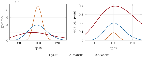
\Gamma=\frac{e^{-qT}\varphi(d_1)}{S\sigma\sqrt T},\quad \mathcal V=Se^{-qT}\varphi(d_1)\sqrt T,\quad \mathrm{Vanna}=-\frac{e^{-qT}\varphi(d_1)\,d_2}{\sigma},\quad \mathrm{Volga}=\mathcal V\,\frac{d_1d_2}{\sigma},

and the put has the same gamma and vega. Desks report Greeks in money: vega per volatility point (0.01), theta per calendar day, rho per basis point, and gamma through the next quantity.

Definition 4.2 (Cash gamma and straddle)

The cash gamma of a position is $\tfrac12\Gamma S^2$ : the P&L of the delta-hedged position per unit of squared return, since $\tfrac12\Gamma\,dS^2=\tfrac12\Gamma S^2(dS/S)^2$ . Risk reports also give $\Gamma S^2/100$ , the change of the cash delta $\Delta S$ for a 1% move. A straddle is a call and a put with the same strike and expiry: at the money its delta is close to zero and its gamma and vega are twice the call’s.

Gamma (left) and vega per volatility point (right) of a call struck at 100 (=20\%, r=0) at three expiries. Short options concentrate gamma near the strike; long options carry the vega. Both are positive for every long option. Data: the chapter’s code. — **Figure 4.1.** Gamma (left) and vega per volatility point (right) of a call struck at 100 ( $\sigma=20\%$ , $r=0$ ) at three expiries. Short options concentrate gamma near the strike; long options carry the vega. Both are positive for every long option. Data: the chapter’s code.

4.2 The gamma–theta identity and the hedging P&L

Proposition 4.3 (Gamma–theta identity)

The value of any European claim in the Black–Scholes model satisfies

\Theta+\tfrac12\sigma^2S^2\Gamma=r(V-S\Delta)+qS\Delta .

With zero rates and dividends, $\Theta=-\tfrac12\sigma^2S^2\Gamma$ : a long option loses in time exactly what its gamma earns when the share moves by one standard deviation.

Proof. Rearrange the Black–Scholes equation of chapter 3. ∎

Now hold the option priced and hedged at a volatility $\sigma$ , while the share moves as it will. Over a short interval the position (option, $-\Delta$ shares, cash financing both) changes by a Taylor expansion in which the delta term is hedged away:

d\Pi=\Theta\,dt+\tfrac12\Gamma\,dS^2-r(V-S\Delta)\,dt-qS\Delta\,dt =\tfrac12\Gamma S^2\Bigl(\bigl(\tfrac{dS}{S}\bigr)^2-\sigma^2dt\Bigr),

by the identity. This is the whole theory of a volatility book in one line.

Definition 4.4 (Hedging P&L)

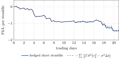
The hedging P&L of a delta-hedged option is the change of value of the option together with its hedge and its financing. For a long option hedged at volatility $\sigma$ it is, to second order over each interval, the cash gamma times the difference between the squared return and the variance the hedge assumed:

\pnl_{[0,T]}=\int_0^Te^{r(T-t)}\tfrac12\Gamma_tS_t^2\bigl(\sigma_{\mathrm{real},t}^2-\sigma^2\bigr)dt ,

where $\sigma^2_{\mathrm{real},t}dt=(dS_t/S_t)^2$ is the instantaneous realised variance.

The formula says three things. The P&L is paid at the rate of the cash gamma, so moves on days when gamma is large count more than moves on days when it is small. It is quadratic in returns and blind to their sign. And it involves realised variance, not realised volatility, a fact that chapter 14 turns into a product.

Proposition 4.5 (Expected hedging P&L)

If the share follows the Black–Scholes model with volatility $\sigma_{\mathrm{real}}$ and the option is sold at $\sigma$ and hedged continuously at $\sigma$ , the expected hedging P&L of the long option (with the drift at $r$ ) is $V(\sigma_{\mathrm{real}})-V(\sigma)$ in present value.

Proof. The present value of the P&L is $\E\bigl[\int_0^Te^{-rt}\tfrac12\Gamma_t(\sigma)S_t^2 (\sigma_{\mathrm{real}}^2-\sigma^2)dt\bigr]$ . The function $u=V(\sigma_{\mathrm{real}})- V(\sigma)$ solves the pricing equation at $\sigma_{\mathrm{real}}$ with the source term $\tfrac12(\sigma_{\mathrm{real}}^2-\sigma^2)S^2\Gamma(\sigma)$ and zero terminal value; the Feynman–Kac formula (One Quant Book 4, chapter 4) gives the claim. ∎

Example 4.6 (The desk’s month)

The one-month at-the-money straddle on a share at 100 is worth 4.6059 at 20 volatility and 5.7570 at 25, with zero rates. A desk short 1 000 straddles (multiplier 100) expects to lose $(5.7570-4.6059)\times100\,000$ , about USD 115 100, when realised volatility comes in at 25. Its vega, 0.2302 per point per straddle, times five points gives nearly the same number: for small changes the expected loss is vega times the volatility gap.

Figure 4.2. One month of a short straddle sold at 20 volatility, hedged four times a day, while the share realises 25. The dashed line adds the gamma–theta terms interval by interval; it never strays more than 0.09 from the book’s P&L and ends 0.04 from it. The P&L falls in steps on the days with large moves and drifts up on quiet days, when theta wins. Data: the tutorial.

4.3 Discrete hedging error

The identity is exact only in the limit of continuous hedging. A desk that hedges once a day holds a stale delta between rebalancings, and the squared return over a day is a noisy estimate of the day’s variance.

Definition 4.7 (Discrete hedging error)

The discrete hedging error is the difference between the terminal value of an option hedged at $N$ dates and that of the same option hedged continuously, when realised volatility equals the hedging volatility. Its mean is close to zero and its standard deviation falls like $1/\sqrt N$ .

Proposition 4.8 (Size of the error)

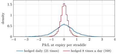
For an option near the money hedged $N$ times at its implied volatility $\sigma$ , which the share realises, the standard deviation of the hedging error is approximately $\sqrt{\pi/4}\,\mathcal V\sigma/\sqrt N$ .

Partial proof. Over a step the error is $\tfrac12\Gamma S^2(x^2-\sigma^2\Delta t)$ with $x$ the step’s return; its variance is $\tfrac12\Gamma^2S^4\sigma^4\Delta t^2$ for normal returns. Summing the independent steps, $\Delta t=T/N$ , and averaging $\Gamma^2S^4$ over the paths gives the $1/\sqrt N$ rate and the vega scaling; the constant $\sqrt{\pi/4}$ comes from that average for an at-the-money option (Derman and Kamal). ∎

For the one-month straddle hedged daily, the formula gives 0.890 and a simulation of 20 000 paths gives 0.865; hedging eight times a day brings the simulated figure to 0.308 (Figure 4.3). The noise is as large as the edge: a desk that sells volatility two points above what the share will realise earns, on average, twice the vega per straddle, about 0.46, and with daily hedging has a standard deviation of 0.87 around it. Selling volatility is a statistical business, run on many positions.

Figure 4.3. Distribution of the P&L of a short one-month straddle sold at 20 volatility when the share realises exactly 20, over 20 000 simulated paths. Both distributions are centred on zero; their standard deviations, 0.85 and 0.31, fall like one over the square root of the number of hedges. Data: the tutorial.

4.4 Break-even volatility

Definition 4.9 (Break-even volatility)

The break-even volatility of a hedged option is the realised volatility at which, over a period, its gamma P&L exactly pays its theta and financing. The break-even move is the corresponding daily move of the underlying: $\tfrac12\Gamma\,\delta S^2=-\Theta\,\delta t$ .

With zero rates the gamma–theta identity makes the break-even volatility equal to the implied volatility at which the option is marked. For the straddle of the example, theta is $-0.0757$ per calendar day and gamma 0.1381: the break-even move is $\sqrt{2\times0.0757/0.1381}=1.047$ , a day’s standard deviation at 20 volatility over 365 days. Desks that count theta over calendar days but see moves only on trading days need the move on trading days to pay the weekend’s theta as well: over 252 trading days the break-even move is 1.26. The choice of clock is a modelling decision, taken up in chapter 8.

4.5 Which volatility to hedge at

A desk that is sure the share will realise 25 still chooses the volatility in its delta. Two choices are natural.

Proposition 4.10 (Hedging at implied against hedging at realised)

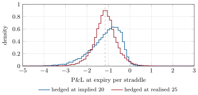
Suppose the option is bought at implied $\sigma$ and the share realises a constant $\sigma_{\mathrm{real}}>\sigma$ . Hedging continuously with the delta at $\sigma_{\mathrm{real}}$ locks in the profit $V(\sigma_{\mathrm{real}})-V(\sigma)$ at inception, but the mark-to-market at implied fluctuates along the way. Hedging with the delta at $\sigma$ makes each day’s P&L a known function of that day’s return $x$ , namely $\tfrac12\Gamma S^2(x^2-\sigma^2\delta t)$ , but the total depends on the path through the gamma weighting; its mean is the same.

Proof. With the delta at $\sigma_{\mathrm{real}}$ , the hedged option is a replicating portfolio for the true model: its terminal value is fixed and equals its value at $\sigma_{\mathrm{real}}$ at inception. With the delta at $\sigma$ , apply Definition 4.4 and Proposition 4.5. ∎

In practice realised volatility is not known in advance, so the second choice is the default: the hedge is at implied, the book’s P&L is explained by gamma, theta and vega every day, and the realised-volatility view is expressed in the size of the position. Figure 4.4 shows both choices on the desk’s month, hedged four times a day: same mean, a standard deviation of 0.72 at implied and 0.54 at realised, the latter being only discrete hedging noise.

Figure 4.4. A short straddle sold at 20 while the share realises 25, hedged four times a day with the delta at 20 or at 25. Both centre on the expected loss

-1.151

(dashed). Hedging at the true volatility removes the path dependence and leaves only the discrete-hedging noise. Data: the tutorial.

Definition 4.11 (Bump-and-reprice)

Bump-and-reprice computes a Greek by repricing the position with one input shifted and taking a finite difference: delta as $(V(S+h)-V(S-h))/2h$ , gamma as $(V(S+h)-2V(S)+V(S-h))/h^2$ , vega with a shift of one volatility point. It works for any pricer, at the cost of two or three valuations per Greek.

The step is a trade-off (One Quant Book 4, chapter 25): too large and the difference measures a chord, not a slope; too small and catastrophic cancellation leaves only rounding noise, especially for gamma. Desks use a relative spot step of about 1% for risk reports, matching the moves they care about, and a smaller one when a smooth derivative is needed. For Monte Carlo pricers the repricings must use the same random numbers, or the noise of two independent estimates swamps the difference (chapter 23).

4.6 Tutorial: a month of hedging

Goal. Simulate the desk’s month in full: sell straddles, hedge on a schedule, compare the P&L with the gamma–theta prediction, and measure the discrete-hedging noise and the effect of the hedging volatility. End state: Figures 4.2, 4.3 and 4.4 and the numbers of the weekend problem.

The simulator, vectorised over 20 000 paths: sell at implied, hedge at a chosen volatility, finance at $r$ , settle the straddle at expiry.

def hedge_short_straddle(n_paths: int, steps: int, t: float = 1 / 12, s0: float = 100.0, k: float = 100.0,
                         r: float = 0.0, vol_imp: float = 0.20, vol_real: float = 0.25,
                         hedge_vol: float | None = None, seed: int = 1, mu: float = 0.0):
    """Sell one straddle at vol_imp, delta-hedge `steps` times at hedge_vol (default: vol_imp) while the
    share realises vol_real. Returns the P&L at expiry per path (in currency, per straddle)."""
    rng = np.random.default_rng(seed)
    hv = vol_imp if hedge_vol is None else hedge_vol
    dt = t / steps
    s = np.full(n_paths, s0)
    c, p, n1, _ = call_put_vec(s, k, t, r, hv)
    premium = bs(s0, k, t, r, 0.0, vol_imp, "C") + bs(s0, k, t, r, 0.0, vol_imp, "P")
    delta = 2 * n1 - 1                       # straddle delta; the short position holds +delta shares
    cash = premium - delta * s
    for i in range(1, steps + 1):
        z = rng.standard_normal(n_paths)
        s = s * np.exp((mu - 0.5 * vol_real ** 2) * dt + vol_real * math.sqrt(dt) * z)
        cash = cash * math.exp(r * dt)
        tau = t - i * dt
        if i < steps:
            _, _, n1, _ = call_put_vec(s, k, tau, r, hv)
            new = 2 * n1 - 1
            cash -= (new - delta) * s
            delta = new
    return cash + delta * s - np.abs(s - k)

Listing 4.1. Delta-hedging a short straddle on many paths at once. code/derivatives/04-greeks-and-the-hedging-pnl/python/dv_greeks.py

Greeks in desk units by bump-and-reprice, for any pricer:

def bump_greeks(pricer: Callable[..., float], params: dict, h_spot: float = 0.01, h_vol: float = 0.01,
                h_rate: float = 1e-4, days: float = 1.0) -> dict[str, float]:
    """Central differences for delta, gamma, vega, rho; a forward roll of `days` for theta."""
    s, v0 = params["spot"], pricer(**params)

    def at(**kw) -> float:
        return pricer(**{**params, **kw})
    up, dn = at(spot=s * (1 + h_spot)), at(spot=s * (1 - h_spot))
    delta = (up - dn) / (2 * h_spot * s)
    gamma = (up - 2 * v0 + dn) / (h_spot * s) ** 2
    vega_pt = (at(vol=params["vol"] + h_vol) - at(vol=params["vol"] - h_vol)) / 2 * (0.01 / h_vol)
    rho_bp = (at(r=params["r"] + h_rate) - at(r=params["r"] - h_rate)) / 2 * (1e-4 / h_rate)
    theta_day = (at(t=max(params["t"] - days * DAY, 0.0)) - v0) / days
    return desk_units({"value": v0, "delta": delta, "gamma": gamma}, s) | {"vega_pt": vega_pt, "rho_bp": rho_bp,
                                                                          "theta_day": theta_day}

Listing 4.2. Central bump-and-reprice Greeks, reported per point, per day and per basis point. code/firm/greeks/firm_greeks.py

Run dv_greeks.problem() and fig_greeks.py; compare the simulated standard deviations with Proposition 4.8.

What to change next. Add a bid–ask cost on every hedge trade and find the hedging frequency that minimises cost plus noise; then let volatility be 25 in the first half of the month and 15 in the second, and compare the P&L of a straddle struck at 100 on paths that end at 100 and at 110.

4.7 Build: the Greek calculator

Purpose. Every position of the miniature firm reports the same Greeks in the same units, whatever pricer values it; the next day’s P&L is predicted from them, so that the unexplained part can be monitored (chapter 25).

Interface. bump_greeks(pricer, params, h_spot, h_vol, h_rate, days) with pricer(**params); desk_units(greeks, spot); predict_pnl(greeks, d_spot, d_vol_pts, days); hedging_pnl(cash_gamma, ret, vol, dt); breakeven_vol.

Rules. Central differences for delta, gamma, vega and rho; theta by rolling the valuation date one calendar day; units: shares, $\Gamma S^2/100$ , per volatility point, per day, per basis point.

Acceptance tests. code/firm/greeks/tests/: bump-and-reprice equals the analytic Greeks of firm.bs in desk units; the one-day prediction is within one cent of a full revaluation for a 1% move; the break-even volatility equals the implied volatility at zero rates.

Stretch. The same Greeks for a portfolio priced by the Monte Carlo engine of chapter 23, with common random numbers; the pricing library of chapter 28 serves them for any instrument through one call.

Sources and further reading

P. P. Boyle and D. Emanuel, “Discretely adjusted option hedges”, Journal of Financial Economics 8 (1980) 259–282.
E. Derman and M. Kamal, “When you cannot hedge continuously: the corrections of Black–Scholes”, Risk 12 (1999) 82–85.
R. Ahmad and P. Wilmott, “Which free lunch would you like today, sir? Delta hedging, volatility arbitrage and optimal portfolios”, Wilmott (2005) 64–79.
H. E. Leland, “Option pricing and replication with transactions costs”, Journal of Finance 40 (1985) 1283–1301.

4.8 Exercises

Exercise 4.1 ★

Give the delta, gamma, vega per point and theta per day of the one-month at-the-money straddle on a share at 100 at 20 volatility, zero rates.

Solution

Solution of Exercise 4.1.

Delta 0.0230, gamma 0.1381, vega 0.2302 per point, theta $-0.0757$ per calendar day.

Exercise 4.2 ★

Check the gamma–theta identity on the numbers of Exercise 4.1.

Solution

Solution of Exercise 4.2.

With $r=q=0$ : $\Theta=-\tfrac12\sigma^2S^2\Gamma=-\tfrac12\times0.04\times10\,000\times0.1381 =-27.63$ per year, $-0.0757$ per day, as the analytic theta.

Exercise 4.3 ★

A hedged long option has a cash gamma of 5 000 and is marked at 20 volatility. The share moves 2% today. Give the day’s gamma P&L, the theta, and the net (zero rates, one calendar day).

Solution

Solution of Exercise 4.3.

Gamma P&L $5\,000\times0.02^2=2.00$ ; theta $-5\,000\times0.2^2/365=-0.55$ ; net $+1.45$ .

Exercise 4.4 ★★

Why is the hedging P&L blind to the sign of the moves? Give a path on which a long straddle loses money although the share ends far from the strike.

Solution

Solution of Exercise 4.4.

Each interval pays $\tfrac12\Gamma S^2(x^2-\sigma^2\delta t)$ , quadratic in the return $x$ . A share that drifts to 120 in small steps (each below the break-even move) loses theta every day: the long straddle, hedged, loses money although unhedged it would have paid 20 at expiry. The hedge sold the drift away as it happened.

Exercise 4.5 ★★

By how much must the number of hedges grow to halve the discrete-hedging error? What does it cost if each hedge trade pays half a spread?

Solution

Solution of Exercise 4.5.

By four: the error falls like $1/\sqrt N$ . Each trade then rebalances a delta change about half as large, so the total traded quantity, and the cost, grow like $\sqrt N$ : twice the cost for half the noise (the Leland trade-off).

Exercise 4.6 ★★

Using Proposition 4.8, give the standard deviation of the daily-hedging error of the desk’s straddle, and compare it with the simulated 0.865.

Solution

Solution of Exercise 4.6.

$\sqrt{\pi/4}\times23.02\times0.2/\sqrt{21}=0.890$ , within 3% of the simulated 0.865.

Exercise 4.7 ★★★

Coding. With hedge_short_straddle, measure the mean and standard deviation of the P&L when the straddle is sold at 20, the share realises 25 and the hedge is at 25, hedged daily, on seed 1.

Solution

Solution of Exercise 4.7.

Mean $-1.147$ , standard deviation 1.082: the mean is unchanged, and with daily hedges the discrete-hedging noise, not the choice of volatility, dominates the spread.

Exercise 4.8 ★★★

Find the flaw. “Our short straddles made money on 70% of the days this month and lost overall. Theta was on our side; the loss must be a pricing error.”

Solution

Solution of Exercise 4.8.

A short straddle collects theta on most days and pays gamma on the few days with large moves; with realised above implied, the quadratic losses on large-move days exceed the steady gains. A high share of winning days is the signature of selling optionality, not evidence of a pricing error; the loss is the gamma–theta identity at work.

4.9 Problem: The Short-Straddle Month

Problem 4.1

Weekend problem — selling volatility that turned out too cheap

A desk sells 1 000 one-month at-the-money straddles (multiplier 100) on a share at 100, at 20 implied volatility, zero rates and no dividend, and hedges daily. Over the month the share realises 25.

Part I — The position.

Give the premium received, per straddle and in dollars.
Give the position’s delta in shares and the initial hedge.
Give its cash gamma and its gamma per 1% move, per straddle.
Give its vega in dollars per volatility point and its theta per day.
Give the break-even daily move over 365 and over 252 days.

Part II — The expected outcome.

Give the straddle’s value at 25 volatility.
Give the expected loss per straddle and in dollars.
Compare it with five times the vega.
Why do the two agree so closely?
Would the answer change if the desk hedged continuously?

Part III — The simulated month.

Give the simulated mean and standard deviation of the P&L per straddle with daily hedging.
Give the standard deviation with eight hedges a day.
Give the probability of a loss with daily hedging.
Give the mean and standard deviation when the desk hedges at 25 instead of 20.
With realised volatility equal to 20, what are the mean and standard deviation?

Part IV — Judgement.

What would the desk have needed to believe to sell at 20?
How would you size the position so that one bad month does not end the desk?
Which Greek of the report should have warned the desk?
State the named result: the expected loss of the position from the gamma–theta identity and its standard deviation under daily hedging, in dollars.
In one sentence: what does a delta-hedged option pay?

Solution

Solution of Problem 4.1.

1. 4.6059 per straddle; USD 460 595. 2. Each straddle has delta 0.0230; short 1 000 with multiplier 100 is $-2\,303$ shares; the desk buys 2 303 shares. 3. Cash gamma 690.70; gamma per 1% move 13.81 (of cash delta). 4. Vega USD 23 023 per point (short, so a loss when volatility rises); theta USD 7 569 a day in the desk’s favour. 5. 1.047 over 365 days; 1.260 over 252. 6. 5.7570. 7. 1.1510 per straddle; USD 115 104. 8. $5\times0.2302=1.1512$ . 9. The straddle’s value is nearly linear in volatility near the money (volga is small), so vega times the gap is an accurate first-order estimate. 10. No: continuous hedging gives the same expectation, with no dispersion coming from the hedging schedule. 11. Mean $-1.145$ , standard deviation 1.183. 12. 0.620. 13. 87.3%. 14. Mean $-1.147$ , standard deviation 1.082. 15. Mean 0.003, standard deviation 0.865: pure discrete-hedging noise. 16. That the share would realise at most 20 over the month, after costs and with a margin for the hedging noise. 17. Limit the vega (and the gamma near expiry) so that a plausible volatility shock, say ten points, and two standard deviations of hedging noise stay within the monthly loss limit. 18. The vega, read with a scenario for realised volatility, and the gamma concentration near the strike. 19. An expected loss of USD 115 100 and a standard deviation of USD 118 300 with daily hedging. 20. The cash gamma times the difference between realised and implied variance, summed over the life of the option.

4.10 Interview questions

Interview question 4.1 ★ trader

You are long a delta-hedged at-the-money option. The underlying does not move for a week. What happened to your P&L, and why?

Solution

Solution of Interview question 4.1.

It lost a week of theta: the option decayed and no gamma P&L came in to pay for it. By the gamma–theta identity, a hedged long option earns only when the underlying moves more than the implied volatility assumes.

What the interviewer is looking for: theta as the rent for gamma.

Interview question 4.2 ★ trader, researcher

State the gamma–theta relation and explain it without formulas.

Solution

Solution of Interview question 4.2.

$\Theta\approx-\tfrac12\Gamma S^2\sigma^2$ : the time decay of a hedged option is exactly what its gamma earns if the underlying moves by one standard deviation of the implied volatility each day. Being long gamma means paying theta for convexity.

What the interviewer is looking for: the identity, and “break-even at implied”.

Interview question 4.3 ★★ researcher

Derive the P&L of a delta-hedged option over one day in terms of its gamma and the realised and implied volatilities.

Solution

Solution of Interview question 4.3.

Taylor-expand the option: $\Theta\delta t+\Delta\delta S+\tfrac12\Gamma\delta S^2$ ; the hedge removes $\Delta\delta S$ ; the identity replaces $\Theta$ by $-\tfrac12\Gamma S^2 \sigma_{\mathrm{imp}}^2$ (zero rates): P&L $=\tfrac12\Gamma S^2\bigl((\delta S/S)^2- \sigma_{\mathrm{imp}}^2\delta t\bigr)$ .

What the interviewer is looking for: the second-order expansion and the cancellation.

Interview question 4.4 ★★ trader

You are sure realised volatility will be higher than implied. Should you delta-hedge at implied or at your forecast? What changes?

Solution

Solution of Interview question 4.4.

At your forecast, if it is right, the P&L at expiry is locked in, but the daily mark-to-market swings; at implied, daily P&L is explained by gamma and theta, but the total depends on where the large moves happen relative to the strike. Hedging at implied is the default because the forecast is uncertain and because risk reports and limits are in implied terms.

What the interviewer is looking for: the two properties, and why desks choose implied.

Interview question 4.5 ★★ developer, risk

Your bump-and-reprice gamma is noisy for a Monte Carlo pricer and wrong for a digital near expiry. Why, and what do you do?

Solution

Solution of Interview question 4.5.

Monte Carlo: the up and down repricings use independent random numbers, so their difference is noise divided by $h^2$ ; use common random numbers, pathwise or likelihood-ratio estimators (chapter 23). Digital near expiry: the payoff is discontinuous, gamma is a spike narrower than the bump, and the difference measures the bump size; report gamma over a bump that matches the risk horizon, and manage the digital by a call spread (chapter 15).

What the interviewer is looking for: noise from independent draws, and non-smooth payoffs.

Interview question 4.6 ★★★ researcher, trader

Two books have the same vega and the same realised-minus-implied volatility over a month. Why can their P&Ls differ, and by how much?

Solution

Solution of Interview question 4.6.

Vega sums gamma over the life of the options, but the P&L weights each day’s realised variance by that day’s cash gamma. A book whose gamma sat at strikes the spot visited on its volatile days earns more than one whose gamma sat elsewhere; the difference can be of the order of the whole expected P&L, as the dispersion of Figure 4.4 shows.

What the interviewer is looking for: gamma weighting in time and in spot.

Terms defined in this chapter

See all 2333 terms in the glossary