13Jumps and Lévy Models

A biotechnology company will publish the results of its main clinical trial on Thursday. Its one-week at-the-money options trade at an implied volatility of 160%. No one believes the share will diffuse at 160% a year. It will drift at its ordinary 35% until Thursday, then jump up about 22% or down about 15%, and drift again. A diffusion needs one enormous volatility to reach the same price, and it then misprices every other strike and every other expiry and gives the wrong hedge. A model with a jump needs the one number the desk actually has an opinion on, the size of the move. This chapter covers the evidence that index and single-stock options contain jumps and the three jump-diffusion models in use, Merton’s, Kou’s and Bates’s. It then turns to the pure-jump Lévy models, to what no hedge in the underlying can remove, and to the situations in which jumps change the price of a trade.

13.1 Why diffusions fail at short expiries

In a diffusion, however volatile, the price moves continuously. Over a short time $T$ its log-return is approximately normal with standard deviation $\sigma\sqrt T$, so an option struck a fixed distance out of the money needs a move of many standard deviations to pay off. Its price falls faster than any power of $T$ as the expiry shrinks: the normal tail $e^{-k^2/(2\sigma^2T)}$ decays exponentially in $1/T$. With jumps, a single jump can carry the price past the strike at any time. The probability of one jump before $T$ is about $\lambda T$ for a jump intensity $\lambda$, so the option’s price is proportional to $T$ for small $T$:

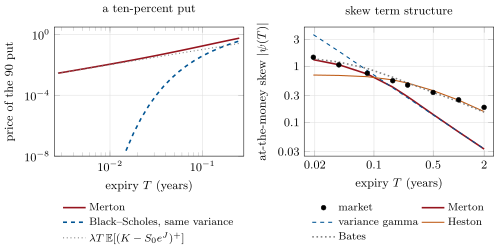
with $J$ the log-size of a jump. At the money both components contribute. The diffusion gives a price proportional to $\sqrt T$, which dominates. Carr and Wu turned the difference in these speeds into a test of what kind of process underlies the options, and found on S&P 500 options both a continuous component and a jump component.

Example 13.1 (A ten-percent put as expiry shrinks)

Take the Merton model fitted below to chapter 9’s surface ($\sigma=9.8\%$, $\lambda=3.16$ jumps a year of mean log-size $-5.8\%$). Its ten-percent out-of-the-money put, divided by its expiry, tends to $\lambda\E[(K-S_0e^J)^+]=1.00$ a year: at one day the ratio is 1.02. Under Black–Scholes with the same total variance, 16.4% a year, the same put is worth $3\times10^{-36}$ at one day and $6\times10^{-9}$ at five days (Figure 13.1, left).

The same argument explains the smile. A diffusion’s short-dated implied volatility is flat, because its short-dated distribution is normal. A jump’s is steep, because its short-dated distribution is a mixture of “nothing happened” and “one jump happened”, with fat tails. For a Lévy process, the class that contains every model of this chapter except Bates’s, the cumulants of the log-return all grow linearly in $T$. The skewness therefore scales like $T^{-1/2}$ and the excess kurtosis like $T^{-1}$. The smile is steepest at short expiries and fades as the central limit theorem takes over.

13.2 Jump-diffusions: Merton, Kou, Bates

A jump-diffusion adds to the Brownian motion of chapter 3 a compound Poisson process (One Quant Book 4, chapter 6): jumps arrive at rate $\lambda$ and each multiplies the price by $e^{J}$, with the $J$ independent and identically distributed. To keep the discounted price a martingale, the drift is lowered by the expected relative jump, $\lambda\bar k$ with $\bar k=\E[e^J]-1$. With $x_T=\ln(S_T/F_T)$ and $\phi_J$ the characteristic function of $J$, every such model has

the Lévy–Khintchine form (Book 4, chapter 6) with a Gaussian part and a finite jump measure. The three models differ in the law of $J$, and in whether the volatility is itself random.

Definition 13.2 (Merton jump-diffusion model)

The Merton jump-diffusion model is the jump-diffusion with normal log-jumps, $J\sim\mathcal N(\mu_J,\delta^2)$, so $\phi_J(u)=e^{iu\mu_J-\frac12\delta^2u^2}$ and $\bar k=e^{\mu_J+\frac12\delta^2}-1$. Its parameters are $(\sigma,\lambda,\mu_J,\delta)$.

Merton’s model has a closed-form price. Condition on the number $n$ of jumps before $T$, which is Poisson with mean $\lambda T$. Given $n$, the log-return is normal, so the option is a Black price with a shifted forward and a larger variance:

The tutorial checks it against the Fourier price of chapter 10’s integral to a few millionths.

Definition 13.3 (Kou model)

The Kou model is the jump-diffusion with double-exponential log-jumps: with probability $p$ the jump is up and exponential with rate $\eta_1>1$, otherwise down and exponential with rate $\eta_2$, so $\phi_J(u)=p\,\frac{\eta_1}{\eta_1-iu}+(1-p)\frac{\eta_2}{\eta_2+iu}$. Its parameters are $(\sigma,\lambda,p,\eta_1,\eta_2)$.

Kou chose the double exponential for two reasons. It gives asymmetric tails that are heavier than normal on each side, and the exponential law is memoryless: the overshoot of a jump over a barrier is again exponential, which yields analytical prices for path-dependent options as well as vanillas. The condition $\eta_1>1$ keeps $\E[e^J]$ finite.

Definition 13.4 (Bates model)

The Bates model is Heston’s stochastic volatility model (chapter 10) with Merton jumps added to the price. The characteristic function is the product of Heston’s and the jump factor, and the parameters are $(v_0,\kappa,\bar v,\eta,\rho,\lambda,\mu_J,\delta)$.

The division of labour is the point of Bates’s model. Jumps make the short-dated skew. Stochastic volatility makes the long-dated skew and the term structure. Neither can do the other’s job: jump skew fades like $T^{-1/2}$, and Heston’s short skew levels off (chapter 10).

Example 13.5 (Three models on one expiry, one on all)

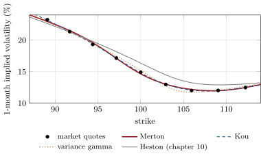
Fitted to the one-month smile of chapter 9’s surface (nine strikes within two standard moves), Merton returns $\sigma=9.8\%$, $\lambda=3.16$, $\mu_J=-5.8\%$, $\delta=4.6\%$ with a root-mean-square error of 0.18 volatility point. Kou returns $\sigma=8.4\%$, $\lambda=11.7$, $p=0.24$, $\eta_1=85$, $\eta_2=30.4$, with an error of 0.06. Variance gamma (next section) has an error of 0.24 (Figure 13.2). Carried to other expiries, all three fail. At one year Merton’s skew is $-0.07$ against the market’s $-0.25$. At one week variance gamma’s is $-3.66$ against $-1.44$ (Figure 13.1). Bates fitted to all eight expiries from one week to two years has an error of 0.34 point, with $v_0=0.018$, $\kappa=2.06$, $\bar v=0.062$, $\eta=0.85$, $\rho=-0.70$ and jumps $\lambda=2.34$, $\mu_J=-3.6\%$, $\delta=3.0\%$. Its skew is $-1.36$ at one week and $-0.23$ at one year.

13.3 Pure-jump Lévy models

A Lévy process with infinitely many small jumps in every interval can do without the Brownian part. The small jumps play the role of the diffusion, and the large ones make the tails. The best known such model changes the clock of a Brownian motion.

Definition 13.6 (Variance gamma model)

The variance gamma model runs a Brownian motion with drift $\theta$ and volatility $\sigma$ on a random clock $g_t$, a gamma process with mean rate one and variance rate $\nu$ (a subordinator, One Quant Book 4, chapter 6): $x_t=\omega t+\theta g_t+\sigma W_{g_t}$, with $\omega$ set so that $\E[e^{x_t}]=1$. Its characteristic function is $\E[e^{iux_t}]=e^{iu\omega t}\bigl(1-iu\theta\nu+\frac12\sigma^2\nu u^2\bigr)^{-t/\nu}$, and $\omega=\frac1\nu\ln\bigl(1-\theta\nu-\frac12\sigma^2\nu\bigr)$.

The three parameters have direct meanings. $\sigma$ sets the scale, $\nu$ the kurtosis (the variability of the clock), and $\theta$ the skewness (the drift that the clock carries). Madan, Carr and Chang found that on S&P 500 data the statistical density was nearly symmetric while the risk-neutral density was negatively skewed with more kurtosis. The skew of index options, on this reading, is a price of downside risk more than a feature of realised returns. Conditioning on the clock gives a closed form. Given $g_T=g$ the log-return is normal, so the call is a Black price averaged over the gamma law of $g$, which the build computes by quadrature and checks against the Fourier price. The CGMY model of Carr, Geman, Madan and Yor generalises variance gamma with a fourth parameter that controls how active the small jumps are. It covers finite and infinite activity, and finite and infinite variation.

Example 13.7 (Moments that fade)

For the Merton model fitted above, the skewness of the log-return is $-2.90$ at one week, $-1.39$ at one month and $-0.40$ at one year, and the excess kurtosis 15.2, 3.5 and 0.29: exactly the $T^{-1/2}$ and $T^{-1}$ laws. The fitted variance gamma model is within a few percent of the same numbers, since both were fitted to the same month. That is why a Lévy model fitted at one expiry cannot fit the others. The market’s skew decays like $T^{-0.44}$ (chapter 12), close to the Lévy exponent $-\frac12$ at short expiries, but at long expiries it is held up by the persistence of volatility, which no Lévy process has.

13.4 What cannot be hedged

A market with jumps of random size is incomplete (chapter 1): the share alone cannot replicate an option. Delta hedging works in a diffusion because over a short interval the option’s value is linear in the move to first order, and the second-order term averages out through gamma and theta. A jump is not small. Over a jump the hedged position gains or loses the option’s convexity on the whole move, $V(Se^J)-V(S)-\Delta S(e^J-1)$, and no choice of $\Delta$ removes it for every $J$ at once.

Example 13.8 (Delta hedging in a world with jumps)

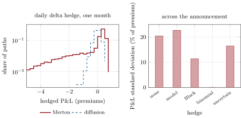
Sell a one-month at-the-money call at the fitted Merton price, 1.89 on a spot of 100, and delta-hedge it daily with Merton’s own delta. Over 20 000 paths the hedged P&L has mean zero and a standard deviation of 0.97 times the premium, and one path in a hundred loses more than 4.1 premiums. In a diffusion with the same total variance, hedged the same way, the standard deviation is 0.185 premiums and the one-in-a-hundred loss 0.50 (Figure 13.3, left). The daily hedge is as good in both worlds between jumps; the difference is the handful of days with a jump.

The scheduled event is the limiting case, and a revealing one. If the outcome has two known sizes, the event is a one-step binomial tree (chapter 2): two states and one hedge instrument, a complete market. The ratio $\Delta^*=\frac{V_u-V_d}{S_u-S_d}$ removes the jump risk entirely. It is not the option’s delta, which measures the response to small moves. Once the sizes are uncertain the tree has more branches than instruments, and a residual remains that only options can hedge.

Example 13.9 (Hedging across the trial result)

The desk is short the biotechnology share’s one-week at-the-money straddle, worth 8.86 on a spot of 50 (a diffusion at 35%, an up move of 22.1% with probability 0.4, a down move of 14.8%). It hedges from just before the announcement to just after. The standard deviation of the P&L across the event is 1.81, or 20.4% of the premium, with no hedge. It is 2.01 with the model’s own delta, $-0.02$, which responds only to small moves. It is 1.01 (11.4%) with the Black delta at the straddle’s implied volatility, $+0.09$. With the binomial ratio, $+0.20$, it is zero. When each outcome’s size is itself uncertain (a standard deviation of 4% in log around each), the best single ratio is still 0.20, but it leaves 1.45, 16.5% of the premium (Figure 13.3, right).

13.5 When jumps matter

Jumps change prices and hedges wherever the payoff is sensitive to large moves over short times.

• Scheduled events. Earnings, trial results, elections, central-bank decisions: the event variance of chapter 8 is a jump. A two-point model reads the probability and sizes from the smile, which a single implied volatility cannot.
• Short-dated out-of-the-money options. Their value is mostly the probability of a jump (Example 13.1); a diffusion calibrated elsewhere makes them nearly free.
• Gap-sensitive payoffs. A barrier monitored continuously (chapter 15) can be crossed by a jump without the price trading near it, so the hedge the desk plans at the barrier never happens. Digitals and autocallables near their triggers, and leveraged products that must be rebalanced, carry the same gap risk.
• Hedging reserves. Where the hedge leaves a jump residual, the price must carry a reserve for it (chapter 27); the size of the residual in Example 13.8 is the order of magnitude.

Where they matter less: long-dated vanillas, whose smile is mostly the dynamics of volatility, and at-the-money options, whose price is mostly the diffusion.

Example 13.10 (Reading the event from the smile)

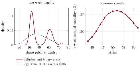
The at-the-money volatility of the biotechnology share, 160.4%, read with chapter 8’s rule against a 35% diffusion, gives an event variance of 0.047. The rule’s standard deviation for the move is then 21.7%, and its expected absolute move is 17.3%. The true move has a standard deviation of 17.6% and an expected absolute size of 17.6%. The straddle prices the expected absolute move, which the rule gets right, while the rule’s standard deviation assumes a normal move and overstates the binary one. A two-point model fitted to the whole smile (Figure 13.4) recovers the probability and both sizes. It does so even when the market’s outcome sizes are uncertain, as the weekend problem shows.

13.6 Tutorial: one interface for jump models

13.7 Build: jump models behind one interface

13.8 Exercises

Exercise 13.1 ★

In Merton’s model with $\lambda=3$ a year, what is the probability of at least one jump in one week (a year of 52 weeks)? In one year?

Solution

Solution of Exercise 13.1.

The number of jumps is Poisson with mean $\lambda T$: $1-e^{-3/52}=5.6\%$ in a week, $1-e^{-3}=95.0\%$ in a year.

Exercise 13.2 ★

Show that $\phi(-i)=1$ for the Merton characteristic function, and say what it means.

Solution

Solution of Exercise 13.2.

At $u=-i$, $iu=1$ and $u^2=-1$, so the exponent is $T\bigl(-\frac12\sigma^2(1-1)-\lambda\bar k+\lambda(e^{\mu_J+\frac12\delta^2}-1)\bigr)=0$. $\phi(-i)=\E[e^{x_T}]=\E[S_T]/F_T$: the model’s forward equals the market’s, the martingale condition that the drift correction $-\lambda\bar k$ enforces.

Exercise 13.3 ★

A Lévy model has skewness $-0.4$ at one year. What is its skewness at one week and at four years?

Solution

Solution of Exercise 13.3.

Skewness scales as $T^{-1/2}$: $-0.4\sqrt{52}=-2.88$ at one week and $-0.4/\sqrt4=-0.20$ at four years.

Exercise 13.4 ★★

Derive the binomial hedge ratio across a two-outcome event, and compute it for the biotechnology straddle from the values after the event: $V_u-V_0=2.21$, $V_d-V_0=-1.48$, moves $+22.1\%$ and $-14.8\%$ on a spot of 50.

Solution

Solution of Exercise 13.4.

Hold $\Delta$ shares against the short straddle; the P&L in each state is $-(V_i-V_0)+\Delta(S_i-S_0)$. Setting the two equal (a riskless position across the event) gives $\Delta^*=(V_u-V_d)/(S_u-S_d)$. Here $(2.21+1.48)/(50\times(0.221+0.148))=3.69/18.45=0.20$.

Exercise 13.5 ★★

Why does the model’s own delta of the straddle, $-0.02$, hedge worse than no hedge at all across the event?

Solution

Solution of Exercise 13.5.

The model delta is the slope of the straddle’s value for a small move of the spot before the event, where the straddle is nearly symmetric: $-0.02$. The event is not a small move; the straddle gains on both outcomes, but more on the up move, so the right hedge is the chord slope $+0.20$. A short position of 0.02 shares adds to the exposure on the up move instead of reducing it.

Exercise 13.6 ★★

Explain why a Lévy model fitted to the one-month smile underestimates the one-year skew, and what Bates adds.

Solution

Solution of Exercise 13.6.

In a Lévy model the skewness decays like $T^{-1/2}$ and the smile flattens quickly, so a fit at one month leaves the one-year skew near zero ($-0.07$ against $-0.25$). The market’s long skew comes from the persistence and correlation of volatility, which Bates adds through Heston’s variance factor; its jumps keep the short end steep.

Exercise 13.7 ★★★

Coding. Re-run the daily hedging experiment with Merton’s jumps halved in size and doubled in frequency ($\mu_J$ and $\delta$ halved, $\lambda$ doubled). How does the standard deviation of the hedged P&L change?

Solution

Solution of Exercise 13.7.

The standard deviation falls from 0.97 to 0.55 premiums, and the one-in-a-hundred loss from 4.1 to 2.1: smaller, more frequent jumps are closer to a diffusion. (The total variance also falls, to 13.5% a year, and the premium to 1.55.)

Exercise 13.8 ★★★

Find the flaw. “The one-week straddle trades at 160% implied volatility. We sold it and delta-hedged with the Black delta at 160%, so our only risk is the difference between realised and implied volatility.”

Solution

Solution of Exercise 13.8.

Most of the 160% is one jump on Thursday, not a diffusion. Across the jump the Black delta leaves a P&L standard deviation of about 11% of the premium even with known outcome sizes, and a hedge adjusted to the jump leaves 16% once the sizes are uncertain. The risk is the size and direction of the move, which only options (or not being short the event) can hedge.

13.9 Problem: The Binary Event

Problem 13.1

Weekend problem — what the one-week smile knows about Thursday

A share trades at 50. Its one-week smile, quoted at 13 strikes from 38 to 62, brackets the publication of trial results. The desk’s model is a diffusion plus one scheduled log-jump: up by $a$ with probability $p$, down by the fair amount otherwise. The “market” is the chapter’s richer model, in which the outcome sizes are themselves uncertain.

Part I — The smile.

1. Give the market’s at-the-money implied volatility and its volatility at the 38 and 62 strikes.
2. Why does the smile fall on both sides of the money?
3. What event variance and standard deviation of the move does chapter 8’s rule read from the at-the-money volatility against a 35% diffusion?
4. What expected absolute move does the rule give, and why is that the more reliable of its two numbers here?
5. Why can no single volatility price all 13 strikes?

Part II — The fit.

6. Fit $(\sigma,p,a)$: give the parameters and the error.
7. Give the implied up and down moves.
8. Why is the fitted diffusion volatility above the true 35%?
9. What does the fitted model say the probability of success is, and how would a trader use that number?
10. What is the fair down move for $p=0.4$ and an up move of $+22.1\%$?

Part III — The hedge.

11. Give the straddle premium and the standard deviation of the unhedged P&L across the event (known sizes).
12. Give the Black delta and the model delta of the straddle, and the P&L standard deviation with each.
13. Give the binomial hedge ratio and the residual with known sizes.
14. Give the best ratio and the residual when the sizes are uncertain, in price and in percent of premium.
15. What instrument would hedge the rest?

Part IV — Judgement.

16. Why is the binomial ratio not the option’s delta?
17. How should the desk hedge in the days before the event, and at the event?
18. What reserve would you hold on a short straddle across the event?
19. State the named result: the jump size and probability implied by the one-week smile, and the error of the delta hedge across the event.
20. In one sentence: what does a jump model give the desk that an implied volatility cannot?

Solution

Solution of Problem 13.1.

1. 159.5% at the money, 79.3% at 38 and 116.4% at 62. 2. The density is bimodal: two humps around the two outcomes, with little mass exactly at the money. Options near the money are expensive relative to a lognormal of the same wings, which is a frown. 3. $1.595^2/52-0.35^2/52=0.0465$; a standard deviation of 21.6%. 4. $21.6\%\times\sqrt{2/\pi}=17.2\%$. The straddle pays the absolute move, so its price measures the expected absolute move whatever the distribution; the standard deviation is read through a normal assumption that a binary move violates. 5. The distribution is not lognormal: one volatility matches one strike’s price, not the shape. 6. $\sigma=40.6\%$, $p=0.399$, $a=0.199$, with an error of 0.07 volatility point. 7. $+22.1\%$ and $-14.7\%$. 8. The uncertainty of the outcome sizes widens each hump; the two-point model can only widen them through the diffusion. 9. About 40%: the market’s price of success. A trader compares it with his own estimate (from trial data, precedents) and trades the difference with digitals or call spreads. 10. $(1-0.4\times1.2214)/0.6-1=-14.8\%$. 11. 8.86; 1.81. 12. $+0.09$ and $-0.02$; 1.01 and 2.01. 13. $0.20$; zero. 14. $0.20$; 1.45, 16.5% of the premium. 15. Options on the event: buying back part of the straddle, or strangles and butterflies that carry the exposure to the outcome sizes. 16. Delta is the response to small moves; the ratio is the chord across the two outcomes. They coincide only for a linear payoff. 17. Delta-hedge the diffusion normally until the event; just before it, move to the chord ratio for the two outcomes; after it, back to the delta. 18. At least the residual of the best hedge, about 1.45 per straddle (one standard deviation), more for a confidence level; scaled by the position and aggregated across events. 19. A success probability of 0.40 with moves of $+22.1\%$ and $-14.7\%$; the Black delta leaves a P&L standard deviation of 1.01 (11.4% of the premium) across the event, the binomial ratio 0.20 removes it with known sizes and leaves 1.45 (16.5%) with uncertain sizes. 20. The distribution of the move, and with it the hedge ratio across the jump, which no single volatility contains.

13.10 Interview questions

Interview question 13.1 ★ trader, researcher

Why do short-dated out-of-the-money options suggest jumps?

Solution

Solution of Interview question 13.1.

In a diffusion a fixed out-of-the-money option needs a move of many standard deviations as $T\to0$, so its price vanishes exponentially fast; with jumps one jump suffices and the price is proportional to $T$. Market prices of short-dated out-of-the-money options decline roughly linearly, and short-dated smiles are steep.

What the interviewer is looking for: the speeds of convergence, and the Carr–Wu idea.

Interview question 13.2 ★ researcher

Write Merton’s jump-diffusion and its price as a series of Black–Scholes prices.

Solution

Solution of Interview question 13.2.

$dS/S=-\lambda\bar k\,dt+\sigma\,dW+(e^J-1)\,dN$, $J\sim\mathcal N(\mu_J,\delta^2)$, $N$ Poisson($\lambda$). Given $n$ jumps the log-return is normal, so $C=\sum_n e^{-\lambda T}(\lambda T)^n/n!\;C_{\mathrm{BS}}(F_n,K,T,\sigma_n)$ with $F_n=Fe^{n(\mu_J+\delta^2/2)-\lambda\bar kT}$ and $\sigma_n^2=\sigma^2+n\delta^2/T$.

What the interviewer is looking for: the compensator, and the conditioning argument.

Interview question 13.3 ★★ trader, risk

Can you delta-hedge a jump? What is left, and how do you hedge it?

Solution

Solution of Interview question 13.3.

No: across a jump the hedged position earns $V(Se^J)-V(S)-\Delta S(e^J-1)$, which no single $\Delta$ removes for all $J$. With two known outcomes a chord ratio does; otherwise hedge the residual convexity with options (they have the same jump exposure), size positions to the residual, and hold a reserve.

What the interviewer is looking for: the convexity over the jump, and options as the hedge.

Interview question 13.4 ★★ researcher

How do skewness and kurtosis scale with maturity in a Lévy model, and what does that imply for the smile?

Solution

Solution of Interview question 13.4.

Cumulants are linear in $T$, so skewness $\propto T^{-1/2}$ and excess kurtosis $\propto T^{-1}$: steep smiles at short expiries that flatten quickly. Index smiles flatten more slowly, which calls for stochastic volatility as well.

What the interviewer is looking for: the scaling, and its consequence.

Interview question 13.5 ★★ developer

Your Fourier pricer is accurate for Heston at one year and wrong for variance gamma at one week. Why?

Solution

Solution of Interview question 13.5.

The variance gamma characteristic function decays only like $|u|^{-2T/\nu}$, very slowly at one week, while Heston’s decays exponentially; a grid truncated at a moderate $u$ loses a large tail. Extend the grid (or use a damped or tail-corrected scheme), and test against the conditional closed form at the shortest expiry.

What the interviewer is looking for: the decay rate of the characteristic function.

Interview question 13.6 ★★★ trader

A share reports earnings tomorrow. How do you price and hedge the one-week straddle, and what can go wrong?

Solution

Solution of Interview question 13.6.

Separate the diffusion from the event: price with a diffusion at the ordinary volatility plus a jump whose law is read from the smile (an event variance, or a two-point fit if the smile shows a frown). Hedge the diffusion with delta before the event and the jump with the chord ratio or with options; after the event, implied volatility collapses to the diffusion. What can go wrong: the size or direction of the move, a move larger than priced, liquidity at the open, and a crush of the other expiries’ volatility.

What the interviewer is looking for: diffusion plus event, the hedge across the jump, the volatility crush.