Derivatives and Volatility · Derivatives

22Trees and Finite-Difference Pricers in Practice

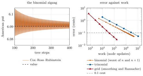
A pricer returns 6.0864 for a one-year American put with a 200-step binomial tree and 6.0975 with 201 steps. The trader asks which to trust. The answer is neither: the true value, to five decimals, is 6.0904, below one and above the other. The Cox–Ross–Rubinstein tree of chapter 2 converges to it, but in a zigzag that alternates with the parity of the step count, and only at first order. At 1 500 steps both neighbours are finally within a tenth of a cent. A Crank–Nicolson grid with the right start-up and the strike on a node gets there with 200 nodes and 200 time steps, 28 times less work. This chapter is about the difference between a pricer that converges and one that is accurate. It covers the pricing equation on a grid, the conditions that dividends and barriers impose, American exercise by a direct algorithm, and how to spend a computing budget.

22.1 The pricing equation on a grid

For one underlying the Black–Scholes equation (chapter 3) is solved most naturally in $x=\ln S$ and in the time to expiry $\tau$ :

\partial_\tau V=\tfrac12\sigma^2\partial_{xx}V+\bigl(r-q-\tfrac12\sigma^2\bigr)\partial_xV-rV.

On a grid $x_0<\dots<x_M$ the derivatives become three-point differences. The build allows the spacing to vary, with $h_\pm$ the distances to the neighbours, so that nodes can be concentrated near the strike where the payoff has its kink. In time the $\theta$ -scheme (One Quant Book 4, chapter 27) mixes explicit and implicit steps. $\theta=\frac12$ is Crank–Nicolson, second-order accurate and unconditionally stable, but not free of oscillations. Each step solves one tridiagonal system, in $O(M)$ operations.

Crank–Nicolson has one known weakness, and option payoffs trigger it. The scheme damps high-frequency components of the solution only weakly. A kinked payoff contains all frequencies, so the first steps leave oscillations near the strike that decay slowly. Prices barely notice them, and gammas do. The standard remedy is Rannacher’s start-up: a few fully implicit half steps first, which damp the high frequencies, then Crank–Nicolson. A second remedy works on the payoff itself.

Definition 22.1 (Payoff smoothing)

Payoff smoothing replaces the payoff’s value at each grid node by its average over the node’s cell, so that the initial condition carries the kink’s effect without its discontinuous derivative; with Rannacher start-up it restores the scheme’s second-order convergence for non-smooth payoffs.

Example 22.2 (Gamma near expiry)

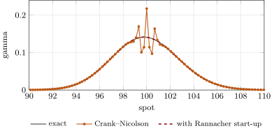
A European put one week from expiry (strike 100, 20% volatility), on a 200-node grid with ten time steps. Plain Crank–Nicolson gives a gamma of 0.217 at the strike, where the exact value is 0.141, and wiggles around the true curve on either side. With two Rannacher start-up steps the largest error is 0.0002 (Figure 22.1). A risk system that reports Crank–Nicolson gammas without the start-up will show hedgers a phantom gamma spike at every strike near expiry.

**Figure 22.1.** Gamma of a one-week put from a 200-node grid and ten time steps. Plain Crank–Nicolson leaves an oscillation at the strike that ten steps cannot damp; two implicit half steps at the start remove it. Data: the tutorial.

Trees are the same equation on a special grid. The binomial tree ties the space step to the time step, $\Delta x=\sigma\sqrt{\Delta t}$ , and is an explicit scheme. The trinomial tree loosens the tie.

Definition 22.3 (Trinomial tree)

A trinomial tree moves the log-price up, down or not at all at each step, by $\Delta x$ (for instance $\sigma\sqrt{3\Delta t}$ ), with probabilities chosen to match the mean and variance of the log-return; it is an explicit finite-difference scheme with a stability condition built into its geometry, and its extra middle branch lets the node grid be placed more freely than a binomial tree’s.

22.2 Discrete dividends and jump conditions

A cash dividend $D$ paid at $t_d$ makes the share fall by $D$ on the ex-date while the option’s value is continuous, since nothing is paid to its holder. The grid enforces this through a condition between the two sides of the date.

Definition 22.4 (Jump condition)

A jump condition links a pricing equation’s solution across a date at which the state variable jumps deterministically: for a cash dividend, $V(t_d^-,S)=V(t_d^+,S-D)$ , applied on the grid by interpolation, followed by a fresh Rannacher start-up, since the interpolated profile is no longer smooth where American exercise bites.

A tree cannot do this directly: shifting a recombining tree’s nodes by a cash amount stops it recombining, which is why chapter 5 used the escrowed model. The grid has no such problem.

Example 22.5 (A three-unit dividend in six months)

With a dividend of 3 paid at six months, the one-year European put is worth 6.835 on the grid, against 6.719 from Black–Scholes on the spot less the dividend’s present value, the escrowed approximation at the same volatility. The American put is worth 7.407, against 6.090 without the dividend.

22.3 Barriers and grid alignment

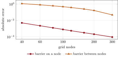
A continuously monitored barrier is a boundary condition: the option is worth zero, or its rebate, at the barrier. The grid must therefore have a node exactly at the barrier. If the barrier falls between nodes, the pricer either moves it to the nearest node, which is a first-order error in the barrier level, or interpolates, which works only approximately. The stretched grid of the build starts at the barrier and concentrates nodes at the strike. Discretely monitored barriers are applied as a projection at the monitoring dates (chapter 15’s shift is the analytical counterpart).

Example 22.6 (Aligned and misaligned)

A one-year down-and-out call (strike 100, barrier 90) is worth 8.665 in closed form. With the barrier on a node, the grid’s error is 0.0049 with 40 nodes and 0.0002 with 200. With uniform grids on which the barrier falls between nodes, the error is 1.10 with 40 nodes, 0.16 with 200 and 0.046 with 300 (Figure 22.2): hundreds of times worse at the same cost, and dependent on where the barrier happens to fall between two nodes.

**Figure 22.2.** Error of a one-year down-and-out call (strike 100, barrier 90) on grids of increasing size, with the barrier exactly on a node and between nodes. Alignment, not size, decides the accuracy. Data: the tutorial.

22.4 American exercise

Early exercise turns the pricing equation into a free-boundary problem (chapter 6): $V\ge g$ , the exercise value, everywhere, with the equation holding where $V>g$ . On a grid, the naive treatment solves the linear system and then takes the maximum with $g$ . That works with an implicit step, and it costs Crank–Nicolson its accuracy, because the projection and the solve are not consistent. Iterative methods such as projected successive over-relaxation solve the constrained system properly, at many times the cost. For a put, whose exercise region is a single interval of low spots, there is a direct method.

Definition 22.7 (Brennan–Schwartz algorithm)

The Brennan–Schwartz algorithm solves a tridiagonal system with the constraint $V\ge g$ exactly when the exercise region is an interval at one end of the grid: it eliminates from the other end, then back-substitutes towards the exercise region, taking the maximum with $g$ at each node; its cost is that of one tridiagonal solve.

The order of elimination is the whole trick. For a put the exercise region lies at low spots, so the elimination runs from the top of the grid down, and the back substitution runs upwards from the exercise region. There each value is fixed by the constraint before the continuation values above it are computed. For a call on a dividend-paying share the order reverses.

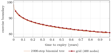
The grid also gives the exercise boundary as a by-product: the highest spot at which the value equals the exercise value, at each date, refined between nodes. The tree gives it too, but only as a staircase of its own nodes (Figure 22.3). For the one-year put the grid places the boundary at 80.85 one year before expiry, while a 2 000-step tree’s boundary jumps between 80.68 and 81.04 from one step to the next.

**Figure 22.3.** The American put’s exercise boundary (strike 100, 5%, 20%) by time to expiry: exercise below the curve. The tree’s boundary is a staircase of its nodes; the grid’s, refined between nodes, is smooth. Data: the tutorial.

22.5 Accuracy against speed

Every pricer has two dials, the grid and the time steps, and a budget. The question the trader asked in the introduction is really this: how much computation buys a given accuracy?

Example 22.8 (A tenth of a cent)

The one-year American put (spot and strike 100, rate 5%, volatility 20%) is worth 6.0904, from a Richardson-extrapolated grid (1 600 and 800 nodes and steps). The Cox–Ross–Rubinstein tree’s error alternates in sign with the parity of the step count. Its two neighbours are both within 0.1 cent from 1 500 steps, 1 125 750 node updates. The trinomial tree converges without the zigzag but at first order: its error is 0.11 cent at 1 600 steps and 0.054 at 3 200. The grid, with a node on the strike, payoff smoothing and Rannacher start-up, errs by 1.04 cent with 50 nodes and steps, 0.30 with 100, 0.091 with 200 and 0.029 with 400: second order. It is within 0.1 cent at 200, 40 600 node updates. That is 28 times less work than the tree (Figure 22.4). Without smoothing and start-up the grid errs by 0.125 cent at 200.

A one-year American put. Left: the Cox–Ross–Rubinstein tree against the value, by number of steps. Right: absolute error in cents against work, in node updates, for the binomial tree (the larger error of each pair n, n+1), the trinomial tree and the Crank–Nicolson grid. Data: the tutorial. — **Figure 22.4.** A one-year American put. Left: the Cox–Ross–Rubinstein tree against the value, by number of steps. Right: absolute error in cents against work, in node updates, for the binomial tree (the larger error of each pair $n$ , $n+1$ ), the trinomial tree and the Crank–Nicolson grid. Data: the tutorial.

Work in node updates is a fair proxy for run time between methods written in the same language, and the grid’s per-node work (a tridiagonal solve) is a few times the tree’s (a weighted average), so the real speed-up is smaller than 28, though of the same order. Two further economies follow from second-order convergence. Richardson extrapolation (Book 4) of two grid sizes cancels the leading error term. Grid stretching puts the nodes where the payoff has its kink. The build carries both. Trees keep a place where their simplicity matters more than their cost: teaching, checking, and products whose early-exercise rules are easiest to state node by node.

22.6 Tutorial: a finite-difference engine

Goal. Build a Crank–Nicolson pricer on a stretched log-spot grid with Rannacher start-up, payoff smoothing, dividend jump conditions, barrier boundaries and American exercise by Brennan–Schwartz; compare it with the trees on error against work. End state: the four figures and the numbers of the weekend problem.

The operator on a non-uniform grid: three-point differences with unequal spacings:

def _operator(x: np.ndarray, r: float, q: float, vol: float):
    """Tridiagonal coefficients (lower, diagonal, upper) of L V at interior nodes on a non-uniform grid."""
    hm, hp = np.diff(x)[:-1], np.diff(x)[1:]
    nu = r - q - 0.5 * vol * vol
    d2 = vol * vol
    lo = d2 / (hm * (hm + hp)) - nu * hp / (hm * (hm + hp))
    di = -d2 / (hm * hp) + nu * (hp - hm) / (hm * hp) - r
    up = d2 / (hp * (hm + hp)) + nu * hm / (hp * (hm + hp))
    return lo, di, up

Listing 22.1. Tridiagonal coefficients of the pricing operator. code/firm/fdpricer/firm_fdpricer.py

Brennan–Schwartz: eliminate from the top, back-substitute upwards with the constraint:

def _brennan_schwartz(a, b, c, d, g):
    """Solve the tridiagonal system with the constraint V >= g for a put-like exercise region at low spots:
    eliminate from the top of the grid down, then back-substitute upwards projecting onto V >= g."""
    n = len(d)
    bp, dp = [0.0] * n, [0.0] * n
    bp[-1], dp[-1] = b[-1], d[-1]
    for i in range(n - 2, -1, -1):
        f = c[i] / bp[i + 1]
        bp[i] = b[i] - f * a[i + 1]
        dp[i] = d[i] - f * dp[i + 1]
    out = [0.0] * n
    out[0] = max(dp[0] / bp[0], g[0])
    for i in range(1, n):
        out[i] = max((dp[i] - a[i] * out[i - 1]) / bp[i], g[i])
    return out

Listing 22.2. The Brennan–Schwartz solver. code/firm/fdpricer/firm_fdpricer.py

The time loop: Rannacher half steps, Crank–Nicolson, boundaries, dividends:

    while step < n_t:
        if implicit_half > 0:
            h, theta = 0.5 * dt, 1.0
            implicit_half -= 1
        else:
            h, theta = dt, 0.5
        tau += h
        rhs = v[1:-1] + (1 - theta) * h * (lo * v[:-2] + di * v[1:-1] + up * v[2:])
        a = list(-theta * h * lo)
        b = list(1 - theta * h * di)
        c = list(-theta * h * up)
        vl = lower(tau, s[0]) if lower else float(v[0])
        vu = upper(tau, s[-1]) if upper else float(v[-1])
        rhs = list(rhs)
        rhs[0] -= a[0] * vl
        rhs[-1] -= c[-1] * vu
        a[0], c[-1] = 0.0, 0.0
        inner = _brennan_schwartz(a, b, c, rhs, list(g[1:-1])) if american else _thomas(a, b, c, rhs)
        v = np.concatenate([[vl], inner, [vu]])
        if american:
            v = np.maximum(v, g)
        if abs(tau - (step + 1) * dt) < 1e-12 * max(1.0, t):
            step += 1
            if step in div_steps:                               # crossing a dividend date backwards
                dcash = div_steps[step]
                v = np.interp(np.maximum(s - dcash, s[0]), s, v)
                if american:
                    v = np.maximum(v, g)
                implicit_half = 2 * rannacher

Listing 22.3. The theta-scheme time loop with jump conditions. code/firm/fdpricer/firm_fdpricer.py

The C++20 twin of the solver, tested against the Python numbers to rounding (the Rust twin has the same algorithm):

// Tridiagonal solve with V >= g, eliminating from the top and projecting on the way up.
inline std::vector<double> brennan_schwartz(const std::vector<double>& a, const std::vector<double>& b,
                                            const std::vector<double>& c, const std::vector<double>& d,
                                            const std::vector<double>& g) {
    const std::size_t n = d.size();
    std::vector<double> bp(n), dp(n), out(n);
    bp[n - 1] = b[n - 1];
    dp[n - 1] = d[n - 1];
    for (std::size_t k = n - 1; k-- > 0;) {
        const double f = c[k] / bp[k + 1];
        bp[k] = b[k] - f * a[k + 1];
        dp[k] = d[k] - f * dp[k + 1];
    }
    out[0] = std::max(dp[0] / bp[0], g[0]);
    for (std::size_t i = 1; i < n; ++i) out[i] = std::max((dp[i] - a[i] * out[i - 1]) / bp[i], g[i]);
    return out;
}

Listing 22.4. Brennan–Schwartz in C++20. code/firm/fdpricer/cpp/firm_fdpricer.hpp

Run dv_fd.accuracy_study(), gamma_profile(), dividend_example(), barrier_alignment() and fig_fd.py.

What to change next. Replace Brennan–Schwartz by solve-then-project with Crank–Nicolson and measure the order of convergence; price the American call with the dividend and find the grid’s exercise boundary just before the ex-date; time the Python, C++ and Rust versions on the same grid.

22.7 Build: the finite-difference engine

Purpose. The miniature firm’s one-dimensional PDE engine: the finite-difference engine of chapter 28’s pricing library, used for American exercise, barriers, dividends and convertibles (chapter 21); twins in C++20 and Rust for the production path.

Interface. uniform_grid(s0, vol, t, m, width); stretched_grid(s0, k, vol, t, m, width, concentration, lower); solve(payoff, x, t, r, q, vol, n_t, american, rannacher, dividends, smoothing, lower, upper) -> values; value_at(x, v, s0) -> value, delta, gamma; american_put; smoothed_payoff; trinomial(s0, k, t, r, q, vol, n, right, american). C++20 firm::fdpricer::american_put, Rust firm_fdpricer::american_put.

Rules. The strike (and any barrier) is a grid node; Rannacher start-up after expiry and after every discontinuity; American exercise by Brennan–Schwartz where the exercise region is an interval, projected iteration otherwise; every price comes with its convergence check (two grid sizes).

Acceptance tests. code/firm/fdpricer/tests/: European value and delta against Black–Scholes on both grids; the American put converges at second order; the trinomial tree converges; the dividend jump condition against a simulation; a barrier on a node against the closed form; cpp/ and rust/: the twins reproduce the Python engine’s numbers to $10^{-9}$ and converge.

Stretch. Two-dimensional grids (alternating directions) for stochastic volatility; a projected successive over-relaxation fallback; adaptive time steps around dividends.

Sources and further reading

M. J. Brennan and E. S. Schwartz, “The valuation of American put options”, Journal of Finance 32(2) (1977) 449–462.
R. Rannacher, “Finite element solution of diffusion problems with irregular data”, Numerische Mathematik 43(2) (1984) 309–327.
D. M. Pooley, K. R. Vetzal and P. A. Forsyth, “Convergence remedies for non-smooth payoffs in option pricing”, Journal of Computational Finance 6(4) (2003) 25–40.
D. Tavella and C. Randall, Pricing Financial Instruments: The Finite Difference Method (Wiley).

22.8 Exercises

Exercise 22.1 ★

Why does the binomial tree’s price alternate above and below the value as the number of steps changes parity?

Solution

Solution of Exercise 22.1.

The tree’s terminal nodes sit either on the strike or straddle it depending on the parity of $n$ : with the strike on a node the kink is represented one way, between nodes the other, and the discretisation error of the payoff changes sign. The error is of order $1/n$ with a parity-dependent constant.

Exercise 22.2 ★

A grid’s error is 0.30 cent with 100 nodes and 0.091 with 200. Estimate the order of convergence and the error with 400.

Solution

Solution of Exercise 22.2.

$\log_2(0.30/0.091)=1.72$ ; the next halving should give about $0.091/2^{1.72}=0.028$ cent (the grid gives 0.029).

Exercise 22.3 ★

Why can a recombining tree not handle a cash dividend directly, and how does the grid?

Solution

Solution of Exercise 22.3.

A cash dividend shifts every node by the same amount, not the same proportion, so the up-then-down and down-then-up paths no longer meet and the tree stops recombining (its size grows exponentially). The grid is fixed in the spot: it applies $V(t_d^-,S)=V(t_d^+,S-D)$ by interpolation and carries on.

Exercise 22.4 ★★

Using the grid values with 800 and 1 600 nodes and steps, derive the Richardson-extrapolated value for a second-order method.

Solution

Solution of Exercise 22.4.

With $V_h=V+ch^2$ : $V\approx V_{1600}+(V_{1600}-V_{800})/3=6.090331+0.000068/3=6.0903535$ .

Exercise 22.5 ★★

Explain why Brennan–Schwartz must eliminate from the top of the grid for a put.

Solution

Solution of Exercise 22.5.

The back substitution must reach the exercise region first, so that each value there is set by the constraint before the continuation values next to it are computed from it; for a put that region is at the low end, so the substitution runs upwards and the elimination downwards from the top. Eliminating the other way would compute continuation values from unprojected neighbours.

Exercise 22.6 ★★

Why does moving a barrier by half a grid cell produce a first-order error in the price?

Solution

Solution of Exercise 22.6.

The price’s sensitivity to the barrier level is of order one (the derivative of the value with respect to $H$ ), so an error of half a cell, $O(h)$ , in the level is an $O(h)$ error in the price, which dominates the scheme’s $O(h^2)$ .

Exercise 22.7 ★★★

Coding. Price the American put by solving with Crank–Nicolson and projecting afterwards instead of Brennan–Schwartz. Measure the error at 100, 200 and 400 nodes and the order.

Solution

Solution of Exercise 22.7.

Errors of 0.80, 0.35 and 0.16 cent at 100, 200 and 400 nodes: first order (the error halves when the grid doubles), against 0.30, 0.091 and 0.029 with Brennan–Schwartz. Projecting after an unconstrained Crank–Nicolson solve is inconsistent with the scheme.

Exercise 22.8 ★★★

Find the flaw. “Our tree prices the American put to six decimals: we ran it at 2 000 steps and the result did not change in the sixth decimal between runs.”

Solution

Solution of Exercise 22.8.

Repeatability is not accuracy: the tree is deterministic, so it returns the same number every run. At 2 000 steps its error is still of order 0.04 to 0.08 cent and alternates with the parity of the step count; only a convergence study against a better method certifies the digits.

22.9 Problem: Neither 200 Nor 201

Problem 22.1

Weekend problem — how much computation a tenth of a cent costs

A risk system prices a book of one-year American puts (spot and strike 100, rate 5%, volatility 20%) with a 200-step binomial tree. The desk must certify every price to a tenth of a cent.

Part I — The tree.

Give the tree’s price with 200 and 201 steps, and the value.
Give the two errors in cents.
From how many steps are both neighbours within 0.1 cent?
How many node updates is that?
Why is averaging $n$ and $n+1$ not a real fix?

Part II — The grid.

Give the grid’s error with 50, 100, 200 and 400 nodes and steps.
Which size first meets the tolerance, and at what work?
What does the grid lose without payoff smoothing and Rannacher start-up?
Give the trinomial tree’s errors at 1 600 and 3 200 steps.
What would Richardson extrapolation of 100 and 200 nodes give?

Part III — The rest of the book.

The book also holds puts with a dividend of 3 in six months. Give the European and American prices.
And down-and-out calls with a barrier at 90: what goes wrong on a uniform grid?
Which Greek does plain Crank–Nicolson get wrong near expiry, and by how much in the chapter’s example?
Why is work in node updates only a proxy for run time?
How would the C++ twin change the picture?

Part IV — Judgement.

What would you tell the trader who asked which of 200 and 201 to trust?
How would you certify a price’s accuracy in production?
When is a tree still the right tool?
State the named result: the grid size and work at which the American put is within 0.1 cent, for the tree and for the grid, and the speed-up of the grid.
In one sentence: what distinguishes a pricer that converges from one that is accurate?

Solution

Solution of Problem 22.1.

1. 6.0864 and 6.0975; the value is 6.0904. 2. $-0.40$ and $+0.72$ cent. 3. 1 500 (and 1 501). 4. $1500\times1501/2=1\,125\,750$ . 5. The average reduces the zigzag but keeps the first-order error, whose constant is not known in advance; it has no error estimate. 6. 1.04, 0.30, 0.091 and 0.029 cent. 7. 200 nodes and steps: 40 600 node updates. 8. Its error at 200 rises to 0.125 cent, over the tolerance; and its Greeks near the strike oscillate. 9. 0.11 and 0.054 cent. 10. $V_{200}+(V_{200}-V_{100})/3$ , within 0.021 cent of the value. 11. 6.835 European, 7.407 American. 12. The barrier falls between nodes: errors of 0.16 at 200 nodes against 0.0002 with the barrier on a node. 13. Gamma: 0.217 at the strike instead of 0.141 one week from expiry, without Rannacher start-up. 14. A grid node update (a tridiagonal solve) costs a few times a tree node update (a weighted average); the ratio depends on the language and the implementation. 15. It lowers every method’s time by a similar factor, so it does not change which method wins; it moves the whole study to where a million node updates cost milliseconds. 16. Neither: both are about half a cent off, on opposite sides; use a method whose error is known and small, or at least extrapolate. 17. Price at two grid sizes and report the difference as the error estimate; check against closed forms where they exist; keep the strike and barriers on nodes; log the grid used. 18. When simplicity matters more than cost (teaching, a quick check), and when exercise rules are easiest to write node by node. 19. Tree: 1 500 steps, 1 125 750 node updates; grid: 200 nodes and steps, 40 600 node updates; the grid needs 28 times less work. 20. The accurate one has a known, controlled error at the size used; the converging one only promises to get there eventually.

22.10 Interview questions

Interview question 22.1 ★ developer, researcher

Why does Crank–Nicolson produce oscillating Greeks for options near expiry, and how do you fix it?

Solution

Solution of Interview question 22.1.

Crank–Nicolson damps high-frequency error components only weakly; a kinked payoff injects them at the strike, and near expiry there are too few steps for them to decay. Gamma, a second derivative, amplifies them. Fix: a few fully implicit (Rannacher) half steps at the start, and payoff smoothing.

What the interviewer is looking for: weak damping, the kink, and the two remedies.

Interview question 22.2 ★★ developer

How do you price an American put on a finite-difference grid efficiently?

Solution

Solution of Interview question 22.2.

Crank–Nicolson in $\ln S$ with the strike on a node, Rannacher start-up, and the Brennan–Schwartz algorithm for the constrained tridiagonal system (one sweep per step), checked by two grid sizes; not projection after an unconstrained solve, which falls to first order.

What the interviewer is looking for: Brennan–Schwartz and the accuracy details.

Interview question 22.3 ★★ researcher

Compare the convergence of a binomial tree, a trinomial tree and a Crank–Nicolson grid for an American put.

Solution

Solution of Interview question 22.3.

Binomial: first order, with an oscillation between odd and even step counts. Trinomial: first order, smoother. Crank–Nicolson with smoothing, start-up and the strike on a node: second order. For a tenth of a cent the grid needs about 30 times less work than the binomial tree in the chapter’s case.

What the interviewer is looking for: the orders and the oscillation.

Interview question 22.4 ★★ developer

How do you handle a discrete cash dividend and a continuously monitored barrier on a grid?

Solution

Solution of Interview question 22.4.

Dividend: a jump condition at the ex-date, $V(t_d^-,S)=V(t_d^+,S-D)$ , by interpolation, then a Rannacher restart. Barrier: a grid whose boundary (or a node) is exactly at the barrier, with the rebate as the boundary value; discrete monitoring as a projection at the dates.

What the interviewer is looking for: jump condition and alignment.

Interview question 22.5 ★★ risk

How would you validate the numerical accuracy of a production pricer?

Solution

Solution of Interview question 22.5.

Convergence studies at several grid sizes with the observed order compared with theory; agreement with closed forms and with independent methods (a tree, a Monte Carlo); limit tests (zero volatility, far strikes); Greeks’ smoothness; regression tests pinned to certified numbers; and the same checks for the production (C++) and research (Python) versions.

What the interviewer is looking for: order of convergence, independent references, regression.

Interview question 22.6 ★★★ developer, researcher

Your grid pricer for an American call on a dividend-paying share gives a slightly wrong exercise boundary just before the ex-date. Diagnose.

Solution

Solution of Interview question 22.6.

Candidates: the dividend’s jump condition applied at the wrong step or without a Rannacher restart (oscillations near the boundary); interpolation across the ex-date that smears the kink of the exercise value; the Brennan–Schwartz direction not reversed for a call (exercise region at high spots); the ex-date not on the time grid. Check each against a fine grid and a tree with the dividend.

What the interviewer is looking for: the dividend handling and the elimination direction.

Terms defined in this chapter

See all 2333 terms in the glossary