Derivatives and Volatility · Derivatives
23Monte Carlo Pricers in Practice
A Bermudan option on the best of five shares has no finite-difference grid that fits in memory: a hundred points per dimension is ten billion nodes. A Monte Carlo engine prices it in seconds, and gets the exercise decision wrong by design. It estimates the value of waiting from a regression on the simulated paths, which is only an approximation of the true continuation value, so the exercise policy it follows is suboptimal and its price is a lower bound. A good desk therefore reports two numbers, a lower bound from the policy and an upper bound from a dual method, and the gap between them measures how much the regression still misses. This chapter builds the machinery around the Monte Carlo method of One Quant Book 4: simulating the models, early exercise by regression and its dual bound, three ways to compute Greeks, low-discrepancy numbers with the Brownian bridge, and the engineering that turns it into a pricer.
23.1 Simulating the models
Lognormal assets are simulated exactly, date to date. Every other model is discretised, and the error of the scheme is a bias that adds to the statistical error and does not average away. Heston’s variance is the standard hard case. An Euler step can make the variance negative, and truncating it at zero leaves a bias that shrinks only slowly with the step size. Andersen designed a scheme that matches the first two moments of the variance’s exact transition.
Definition 23.1 (Quadratic-exponential scheme)
The quadratic-exponential scheme (QE) simulates Heston’s variance over a step by matching the mean and variance of its exact conditional law: when is small it draws , a scaled non-central square of a normal; when is large, a mixture of a mass at zero and an exponential. The log-price then uses the integrated variance implied by the start and end variances.
Example 23.2 (Euler against QE)
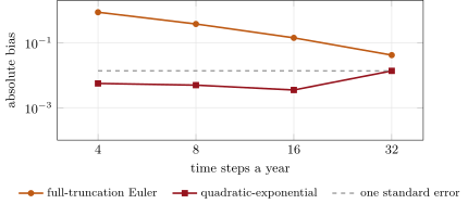
A one-year at-the-money call in chapter 10’s base Heston model (, , , ) is worth 6.751 by Fourier inversion. With 400 000 paths and full-truncation Euler, the bias is 0.857 with 4 steps a year, 0.373 with 8, 0.140 with 16 and 0.041 with 32. With QE the price is within one standard error (0.014) of the exact value at every step count, from 4 steps a year (Figure 23.1). QE saves a factor of ten or more in steps, and so in run time.
23.2 Early exercise by regression
Chapter 6 priced Bermudan and American options backwards on a tree, where the continuation value at each node is an average over its children. A simulation moves forward and has no such average. Longstaff and Schwartz estimated it by regression.
Definition 23.3 (Longstaff–Schwartz method)
The Longstaff–Schwartz method prices a Bermudan option by simulation: working backwards over the exercise dates, it regresses the discounted cash flows that each path realises from the next date on, against a set of basis functions of the state, using the paths that are in the money, and exercises where the exercise value exceeds the fitted continuation value; the policy is then applied to independent paths to give a lower bound.
The price from an estimated policy is biased low, because no policy beats the optimal one. Fitting and pricing on the same paths adds an upward bias, because the regression has seen the paths it then prices. The build fits on one set of paths and prices on another, which keeps the result a lower bound. How low it is depends on the basis. A regression that cannot represent the continuation value leads to exercising at the wrong times.
Definition 23.4 (Dual upper bound)
The dual upper bound of a Bermudan option is for a martingale with and discounted exercise values ; it exceeds the price for every martingale and equals it for the martingale part of the value process. The Andersen–Broadie algorithm builds from a lower-bound policy by nested simulation, so that lower and upper bounds together give an interval for the price.
In the build, the policy’s continuation value is estimated at every outer node by inner paths that follow the policy. With the discounted exercise value where the policy exercises and where it continues, the martingale’s increments are . The inner estimates are noisy, and the maximum in the bound turns noise into an upward bias. The bound is valid for any number of inner paths, but tight only for many.
Example 23.5 (The bias of too few inner paths)
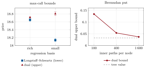
A one-year Bermudan put with ten exercise dates (spot and strike 100, 5%, 20%) is worth 6.0326 on chapter 6’s tree. Longstaff–Schwartz with a cubic basis gives 6.0325 (standard error 0.023). The dual bound on 1 000 outer paths is 6.134 with 100 inner paths per node, 6.054 with 400 and 6.037 with 1 600 (Figure 23.2, right).
Example 23.6 (A three-asset Bermudan max-call)
A call on the best of three independent shares (each at 100, strike 100, volatility 20%, dividend yield 10%, rate 5%), exercisable at nine dates over three years. The basis for the regression is a set of polynomials in the two largest prices, their product, the product of all three and the intrinsic value. With it, Longstaff–Schwartz on 200 000 fresh paths gives 18.649 (standard error 0.039), and the dual bound (1 000 outer paths, 1 000 inner) gives 18.713 (0.019). The gap is 0.064, 0.3% of the price. With a basis of only the largest price and its square, the lower bound falls to 18.137 and the upper rises to 18.805, a gap of 0.668, ten times wider (Figure 23.2, left).
23.3 Greeks: pathwise, likelihood ratio, adjoint
Bumping a Monte Carlo price and repricing gives Greeks with the variance of a difference of two noisy numbers. Common random numbers make the difference far less noisy. Two direct methods, due to Broadie and Glasserman, avoid the bump altogether and give Greeks from the same paths as the price.
Definition 23.7 (Pathwise Greek)
A pathwise Greek differentiates the discounted payoff along each simulated path with respect to the parameter, holding the random numbers fixed, and averages; it requires the payoff to be continuous in the parameter (almost surely differentiable), and fails for digitals and barriers.
Definition 23.8 (Likelihood-ratio Greek)
A likelihood-ratio Greek differentiates the density of the simulated state instead of the payoff: it averages the discounted payoff times the score, the derivative of the log-density with respect to the parameter; it works for discontinuous payoffs, at the cost of a higher variance.
The table compares the two methods on one-year at-the-money options (spot and strike 100, rate 5%, volatility 20%) with 200 000 paths, standard errors in brackets. The last column applies the pathwise method to the digital smoothed into a call spread.
| one year | exact | pathwise | likelihood ratio | smoothed |
|---|---|---|---|---|
| call delta | 0.6368 | 0.6384 (0.0013) | 0.6413 (0.0033) | — |
| call vega | 37.52 | 37.72 (0.17) | 38.24 (0.62) | — |
| digital delta | 0.01876 | 0 (wrong) | 0.01883 (0.00006) | 0.01895 (0.00021) |
| digital vega | 0 (wrong) | (0.010) | (0.007) |
For the call the pathwise estimator’s variance is 6.5 times lower for delta and 13 times lower for vega. For the digital it returns zero, since the payoff’s derivative is zero almost everywhere. The likelihood ratio gets it right. Smoothing the digital into a call spread of half-width one restores a pathwise estimate, at the cost of a bias of the spread’s own.
The pathwise method has an efficient implementation that matters most for large books. Giles and Glasserman’s adjoint method runs the same pathwise calculation backwards along each path: it gives the same values, and its advantage grows with the number of inputs, such as the points of a volatility surface.
Example 23.9 (Twelve vegas for the price of three passes)
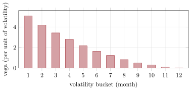
An arithmetic Asian call (one year, 48 steps, strike 100, 20%) is priced along with its sensitivity to the volatility in each of twelve monthly buckets. Forward mode would need one pass per bucket. The adjoint (reverse) pass of One Quant Book 4, chapter 28, runs once backwards along each stored path and accumulates the derivative of the payoff with respect to every step’s state and volatility. It returns all twelve vegas and the delta at a cost of a few forward passes. The price is 5.901 and the delta 0.593. The vega of the first month is 5.064, where bumping that month’s volatility with the same draws gives 5.065, and the vegas fall to 0.016 for the last month (Figure 23.3).
23.4 Bridges and quasi-random numbers
Low-discrepancy sequences (Book 4, chapter 26) fill the unit cube more evenly than random numbers, and for smooth integrands their error falls faster than . A path of dates is a point in dimensions, however, and low-discrepancy sequences lose their advantage in the later coordinates. The Brownian bridge reorders the construction so that the first coordinates carry most of the path’s variance. The first normal sets the endpoint , the second the midpoint given the ends, and so on. The good early coordinates of the sequence then determine the path’s shape.
Example 23.10 (An Asian option with Halton points)
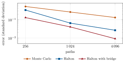
A 16-date Asian call (one year, strike 100, 20%). With 4 096 paths the Monte Carlo standard error is 0.131. Halton points, randomly shifted twenty times to measure their error, give 0.027 with the usual step-by-step construction and 0.0092 with the Brownian bridge, fourteen times smaller than Monte Carlo, the accuracy of about 200 times more random paths. At 256 paths the three errors are 0.53, 0.34 and 0.13 (Figure 23.4).
23.5 Engineering a Monte Carlo pricer
A production engine separates what varies from what is shared. Path generators are one per model: lognormal, local volatility, Heston-QE, stochastic-local. They write paths on a date grid that the product needs, and they never know the payoff. Payoffs read paths only (chapters 16 and 18). Estimators, Longstaff–Schwartz, the Greeks and the dual bound, sit on top. Four rules keep it honest.
- Seeds are data. Every price is reproducible from its seed. Greeks by bumping use the same draws (common random numbers).
- Every number carries its error. The standard error for statistics, a convergence check for the discretisation, and a bound gap for early exercise.
- Variance reduction first. Antithetics, control variates (chapter 16’s geometric Asian), conditioning (chapter 10’s mixing formula) and the bridge usually buy more than extra paths.
- Vectorise over paths, loop over time. The build’s generators are arrays of paths advanced date by date, the natural shape for numpy, for a GPU, and for the adjoint pass that runs back over the same dates.
23.6 Tutorial: bounds, Greeks and bridges
Goal. Price a Bermudan max-call by Longstaff–Schwartz and bound it above by the dual; compute Greeks of a call and a digital by the pathwise and likelihood-ratio methods and bucketed vegas by an adjoint pass; compare Euler and QE for Heston; measure the effect of the Brownian bridge on Halton points. End state: the four figures, the table and the numbers of the weekend problem.
The regression, backwards over the exercise dates, in-the-money paths only:
def lsm_fit(paths: np.ndarray, ex_idx, payoff, basis, k: float, disc: float) -> list:
    """Backward regression of realised continuation values on the basis, in-the-money paths only; returns one
    coefficient vector per exercise date (the last date has none)."""
    cash = payoff(paths[:, ex_idx[-1], :])
    coefs = [None] * len(ex_idx)
    for j in range(len(ex_idx) - 2, -1, -1):
        cash = cash * disc
        s = paths[:, ex_idx[j], :]
        h = payoff(s)
        itm = h > 0
        if itm.sum() > 20:
            x = basis(s[itm], k)
            beta = np.linalg.lstsq(x, cash[itm], rcond=None)[0]
            coefs[j] = beta
            cont = x @ beta
            ex = h[itm] > cont
            idx = np.where(itm)[0][ex]
            cash[idx] = h[itm][ex]
    return coefs
Listing 23.1. Longstaff–Schwartz regression. code/firm/mcpricer/firm_mcpricer.py The dual bound: inner continuation values, martingale increments , the maximum:
def dual_upper(outer: np.ndarray, ex_idx, coefs, payoff, basis, k: float, disc: float, step_sim, n_inner: int,
               seed: int) -> tuple[float, float]:
    """Andersen-Broadie upper bound. For every outer path and exercise date the policy's continuation value
    Q_j is estimated by n_inner inner paths that follow the policy from date j + 1; with L_j = h_j where the
    policy exercises and Q_j where it continues, the martingale increments are L_j - Q_(j-1), and the bound
    is E[max_j (h_j - M_j)] (all discounted to today). step_sim(s, n_steps, rng) simulates n_steps periods."""
    rng = np.random.default_rng(seed)
    n, n_ex = len(outer), len(ex_idx)
    q = np.zeros((n, n_ex + 1))                     # q[:, j] = continuation value at date j (index 0 = today)
    for j in range(n_ex):                           # j = 0 is today, j = 1..n_ex the exercise dates
        start = outer[:, 0 if j == 0 else ex_idx[j - 1], :]
        s = np.repeat(start, n_inner, axis=0)
        alive = np.ones(len(s), bool)
        val = np.zeros(len(s))
        for jj in range(j, n_ex):
            s = step_sim(s, 1, rng)
            h = payoff(s)
            ex = alive & (exercise_now(s, jj, coefs, payoff, basis, k) if jj < n_ex - 1 else h > 0)
            val[ex] = h[ex] * disc ** (jj + 1 - j)
            alive &= ~ex
        q[:, j] = val.reshape(n, n_inner).mean(axis=1) * disc ** j
    m = np.zeros(n)
    best = np.full(n, -np.inf)
    for j in range(1, n_ex + 1):
        s = outer[:, ex_idx[j - 1], :]
        h = payoff(s) * disc ** j
        ex = exercise_now(s, j - 1, coefs, payoff, basis, k) if j < n_ex else payoff(s) > 0
        cont = q[:, j] if j < n_ex else np.zeros(n)
        big_l = np.where(ex, h, cont)
        m = m + big_l - q[:, j - 1]
        best = np.maximum(best, h - m)
    return float(best.mean()), float(best.std() / math.sqrt(n))
Listing 23.2. The Andersen–Broadie upper bound. code/firm/mcpricer/firm_mcpricer.py The adjoint pass for bucketed vegas:
def asian_adjoint(s0: float, k: float, t: float, r: float, vol: float, steps: int, buckets: int, n: int,
                  seed: int) -> dict:
    """Arithmetic Asian call under a volatility with one multiplier per time bucket: the price, the delta and the
    vega of every bucket from one forward and one reverse (adjoint) pass along each path."""
    dt = t / steps
    z = np.random.default_rng(seed).standard_normal((n, steps))
    sig = np.full(steps, vol)
    s = np.empty((n, steps + 1))
    s[:, 0] = s0
    for i in range(steps):                                              # forward pass, stored
        s[:, i + 1] = s[:, i] * np.exp((r - 0.5 * sig[i] ** 2) * dt + sig[i] * math.sqrt(dt) * z[:, i])
    avg = s[:, 1:].mean(axis=1)
    disc = math.exp(-r * t)
    price = disc * np.maximum(avg - k, 0.0)
    sbar = np.zeros((n, steps + 1))
    sbar[:, 1:] = (disc * (avg > k))[:, None] / steps                   # dPayoff/dS_i from the average
    sigbar = np.zeros((n, steps))
    for i in range(steps - 1, -1, -1):                                  # reverse pass
        sigbar[:, i] = sbar[:, i + 1] * s[:, i + 1] * (-sig[i] * dt + math.sqrt(dt) * z[:, i])
        sbar[:, i] += sbar[:, i + 1] * s[:, i + 1] / s[:, i]
    per = steps // buckets
    vegas = np.array([sigbar[:, b * per:(b + 1) * per].sum(axis=1).mean() for b in range(buckets)])
    return {"price": float(price.mean()), "delta": float(sbar[:, 0].mean()), "bucket_vega": vegas}
Listing 23.3. Forward and reverse passes for an Asian call. code/firm/mcpricer/firm_mcpricer.py - Run
dv_mc.bounds(),put_bias(),greek_table(),adjoint(),heston_bias(),qmc_study()andfig_mc.py.
What to change next. Price the max-call with correlation 0.5; add the geometric Asian as a control variate on top of the Halton points; replace the digital’s likelihood ratio by a conditional expectation over the last step (smoothing by conditioning).
23.7 Build: the Monte Carlo engine
Purpose. The miniature firm’s simulation engine: path generators, early exercise with bounds, Greeks by three methods, quasi-random numbers; chapter 28’s Monte Carlo engine wraps it.
Interface. gbm_paths(s0, vols, corr, times, r, q, n, seed); heston_terminal(…, scheme); lsm_fit(paths, ex_idx, payoff, basis, k, disc), lsm_price, exercise_now, max_call_basis, small_basis; dual_upper(outer, …, step_sim, n_inner, seed); call_greeks(…, digital, smooth); asian_adjoint; halton(n, dim, shift), brownian_bridge(z, t), norm_inv.
Rules. Regression and pricing on independent paths; a lower bound is reported with its dual upper bound for every Bermudan; Greeks by pathwise where the payoff is continuous, by likelihood ratio or smoothing where it is not; seeds explicit; no memorised constants in the numerics (the inverse normal is Newton’s method on the error function).
Acceptance tests. code/firm/mcpricer/tests/: the Bermudan bounds bracket the tree value and the dual bound falls with inner paths; pathwise and likelihood-ratio Greeks agree with Black–Scholes and the pathwise digital is zero; the adjoint matches bumping; QE matches the Fourier price; Halton’s first points, the inverse normal and the bridge’s covariances.
Stretch. Sobol points with published direction numbers (cited, not recalled); multilevel Monte Carlo (Book 4); an adjoint pass through Longstaff–Schwartz.
Sources and further reading
- F. A. Longstaff and E. S. Schwartz, “Valuing American options by simulation: a simple least-squares approach”, Review of Financial Studies 14(1) (2001) 113–147.
- L. Andersen and M. Broadie, “Primal-dual simulation algorithm for pricing multidimensional American options”, Management Science 50(9) (2004) 1222–1234.
- L. Andersen, “Simple and efficient simulation of the Heston stochastic volatility model”, Journal of Computational Finance 11(3) (2008) 1–42.
- M. Broadie and P. Glasserman, “Estimating security price derivatives using simulation”, Management Science 42(2) (1996) 269–285.
- P. Glasserman, Monte Carlo Methods in Financial Engineering (Springer, 2003).
- M. Giles and P. Glasserman, “Smoking adjoints: fast Monte Carlo Greeks”, Risk 19 (2006) 88–92; Oxford report NA-05-15 (2005).
23.8 Exercises
Exercise 23.1 ★
Why is a Longstaff–Schwartz price, computed on paths independent of the regression, a lower bound?
Solution
Solution of Exercise 23.1.
The Bermudan’s price is the supremum, over stopping rules, of the expected discounted exercise value. The fitted policy is one stopping rule, so its expected value is at most the price. On paths independent of the fit, the policy is fixed before the paths are drawn, and the average is an unbiased estimate of that policy’s value, which is a lower bound.
Exercise 23.2 ★
Derive the pathwise delta of a call under Black–Scholes, .
Solution
Solution of Exercise 23.2.
, so . The payoff has derivative except at , which has probability zero. The chain rule then gives on each path, and its average is the delta.
Exercise 23.3 ★
Why is the pathwise delta of a digital zero, and why is the likelihood-ratio delta not?
Solution
Solution of Exercise 23.3.
The digital’s payoff is flat on both sides of the strike, so its derivative is zero on almost every path. The delta comes entirely from probability mass crossing the strike, which the pathwise method, differentiating inside the expectation, cannot see; the interchange of derivative and expectation fails for a discontinuous payoff. The likelihood ratio differentiates the density of , which is smooth, and keeps the payoff as it is.
Exercise 23.4 ★★
Derive the likelihood-ratio vega weight for a lognormal terminal price.
Solution
Solution of Exercise 23.4.
is normal with mean and standard deviation . Its log-density is with . Differentiating in with fixed: , so the score is .
Exercise 23.5 ★★
Explain why too few inner paths bias the dual bound upwards, never downwards.
Solution
Solution of Exercise 23.5.
Given the outer path, the inner estimates are the true continuation values plus noise of mean zero. The bound averages , where is what the bound would be with exact values. The maximum is convex, so by Jensen’s inequality . Noise can only raise the bound, and more inner paths shrink the excess, as the put’s 6.134, 6.054 and 6.037 show.
Exercise 23.6 ★★
Why does the Brownian bridge help quasi-random numbers but not pseudo-random ones?
Solution
Solution of Exercise 23.6.
Pseudo-random coordinates are independent and identically distributed. Which normal drives which piece of the path does not change the estimator’s distribution, so the bridge changes nothing. Low-discrepancy coordinates are not all equally good: the first ones are the best spread, and in high dimensions the later ones are poorly spread in pairs. The bridge puts most of the path’s variance into the first coordinates, lowering the effective dimension of the integrand.
Exercise 23.7 ★★★
Coding. Fit and price the max-call’s Longstaff–Schwartz policy on the same paths and compare with the independent-paths price. Explain the sign of the difference.
Solution
Solution of Exercise 23.7.
With 2 000 training paths, averaged over 40 training sets, fitting and pricing on the same paths gives 18.74; the same policies applied to 100 000 independent paths give 18.50. The difference is (standard error 0.06), and the in-sample price is above even the dual upper bound 18.713. The regression has seen each path’s future, so on those paths it exercises with foresight: the bias is upwards. With 200 000 training paths and nine regressors, the bias falls below the noise.
Exercise 23.8 ★★★
Find the flaw. “Our Monte Carlo prices the Bermudan to two cents: the standard error is 0.01.”
Solution
Solution of Exercise 23.8.
The standard error measures only the noise of the lower-bound estimate. The price is biased low by the policy’s suboptimality, and the standard error does not see that bias: with the small basis the standard error is 0.039 but the bounds are 0.668 apart. Two cents needs the dual bound as well (and a check of the time discretisation where the model has one).
23.9 Problem: The Bermudan Bounds
Problem 23.1
Weekend problem — how good is the exercise policy
A desk sells a three-year Bermudan call on the best of three shares (each at 100, strike 100, 20% volatility, 10% dividend yield, rate 5%, nine exercise dates) and prices it by Longstaff–Schwartz.
Part I — The lower bound.
- Give the price with the rich basis and its standard error.
- Why are fitting and pricing done on separate paths?
- Give the price with the small basis (the largest price and its square).
- Which exercise decisions does the small basis get wrong?
- What would a European max-call’s price tell you?
Part II — The upper bound.
- Give the dual bound for the rich basis with 1 000 outer and 1 000 inner paths, and its standard error.
- Give the gap and express it as a share of the price.
- Give the bound and gap for the small basis.
- On the one-asset Bermudan put, how does the bound change with 100, 400 and 1 600 inner paths?
- What does the dual bound cost relative to the lower bound, and why?
Part III — Around the price.
- How would you compute the Bermudan’s delta?
- Why not bump and reprice with fresh paths?
- What does the adjoint method offer for a book of such trades?
- How would quasi-random numbers help, and what limits them here?
- Which discretisation error does this product not have, and which model would introduce one?
Part IV — Judgement.
- Which price would you quote, and which would you book?
- How much reserve would you hold for the exercise policy?
- When would you stop improving the basis?
- State the named result: the gap between the Longstaff–Schwartz lower bound and the dual upper bound for the three-asset Bermudan max-call, and its sensitivity to the regression basis.
- In one sentence: what does the gap between the bounds measure?
Solution
Solution of Problem 23.1.
1. 18.649, standard error 0.039. 2. Pricing on the fitting paths is biased upwards (exercise 7: with 2 000 training paths); independent paths make the price a lower bound. 3. 18.137. 4. It sees only the leader. When the second price is close to the first, the option on the maximum is worth more alive, and the small basis cannot tell those states apart; it exercises too soon there, and too late where the leader is far ahead. 5. 15.57 (standard error 0.07): a lower bound for the Bermudan. The early-exercise premium, about 3.08, comes from the 10% dividend yield, which the holder gives up by waiting. 6. 18.713, standard error 0.019. 7. 0.064, 0.3% of the price. 8. 18.805; the gap is 0.668, ten times wider. 9. 6.134, 6.054 and 6.037 against the tree’s 6.0326: the excess over the tree falls about fivefold each time the inner paths are multiplied by four. 10. Each outer node needs its own inner simulation: inner paths started at each of nine dates, running out to the last date, are 45 million path steps, against 1.8 million for the lower bound’s 200 000 paths, 25 times more. 11. Pathwise, holding the fitted policy fixed: at the optimal policy the value’s sensitivity to the boundary is zero to first order, so fixing it costs little. Or bump with common random numbers and the same policy. 12. The difference of two independent estimates has the variance of both divided by the square of the bump, huge for a small bump. Refitting the policy on new paths adds a jump of its own. 13. All sensitivities (three spots, three volatilities, correlations, rates) of every trade for a cost of a few pricings, independent of their number. 14. The path is a 27-dimensional point (three assets at nine dates); a bridge per asset and a principal-component ordering across assets lower the effective dimension. The exercise decision is a discontinuity, which limits the gain. 15. None in time: lognormal prices are simulated exactly at the exercise dates. Local or stochastic volatility would need small steps between the dates and bring a bias. 16. The desk is short, and the holder may exercise better than the desk’s policy, so the liability is up to the upper bound. Quote around the bounds’ midpoint and book the lower bound with a reserve for the gap. 17. The gap plus about two standard errors of the bounds, per 100 of notional; with the small basis it would be about 0.8. 18. When the gap is within the statistical noise of the bounds: 0.064 against two combined standard errors of 0.086, so the rich basis has reached it. 19. Rich basis: 18.649 against 18.713, a gap of 0.064 (0.3% of the price). Small basis: 18.137 against 18.805, a gap of 0.668, ten times wider. 20. The most the price can be wrong because of the exercise policy, plus the upward bias of the inner simulation.
23.10 Interview questions
Interview question 23.1 ★ developer, researcher
Explain the Longstaff–Schwartz algorithm.
Solution
Solution of Interview question 23.1.
Simulate paths forward. Backwards from the last exercise date, regress the discounted realised cash flows on basis functions of the state, using in-the-money paths, and exercise where the exercise value beats the fitted continuation; carry the realised cash flows back. Then apply the policy to new paths: that price is a lower bound.
What the interviewer is looking for: in-the-money regression, realised cash flows, independent pricing paths, lower bound.
Interview question 23.2 ★★ researcher
How do you get an upper bound for a Bermudan price by simulation?
Solution
Solution of Interview question 23.2.
By duality: the price is at most for any martingale with , with equality for the right one. Andersen–Broadie build from a lower-bound policy with nested simulation of its continuation values. The gap between the bounds measures the policy’s quality.
What the interviewer is looking for: the dual formula, nested simulation, the gap.
Interview question 23.3 ★★ researcher
Compare pathwise and likelihood-ratio Greeks. When does each fail?
Solution
Solution of Interview question 23.3.
Pathwise differentiates the payoff along each path: low variance, but it needs a payoff continuous in the parameter; it fails for digitals and barriers. Likelihood ratio differentiates the density: any payoff, but higher variance (6.5 times for a call’s delta in the chapter), and it needs a known density, awkward after many steps. Smoothing or conditioning mixes the two.
What the interviewer is looking for: continuity versus density, and the variance trade-off.
Interview question 23.4 ★★ developer
How would you simulate the Heston model efficiently, and why not Euler?
Solution
Solution of Interview question 23.4.
Andersen’s quadratic-exponential scheme for the variance, with the integrated variance from both ends of the step for the log-price, and a martingale correction if needed. Euler makes the variance negative when the Feller condition fails, and truncation leaves a bias that decays slowly (0.86 at four steps a year in the chapter, against QE within the noise).
What the interviewer is looking for: QE, and why Euler’s truncation is biased.
Interview question 23.5 ★★ developer, risk
Your Monte Carlo risk is noisy from day to day. What do you change?
Solution
Solution of Interview question 23.5.
Fix the seeds and use the same random numbers for the base and bumped runs; hold the exercise policy fixed; replace bumps by pathwise, likelihood-ratio or adjoint Greeks; smooth discontinuous payoffs; add control variates; check that the noise, not the market, moves the numbers.
What the interviewer is looking for: common random numbers and direct Greeks.
Interview question 23.6 ★★★ developer
Explain adjoint algorithmic differentiation for Monte Carlo Greeks. What does it cost in memory and time?
Solution
Solution of Interview question 23.6.
Run the paths forward and store the states; then run backwards along each path, propagating the derivative of the payoff with respect to each state (the adjoint) and accumulating the sensitivities to every input. All Greeks cost a small multiple of one pricing, whatever their number; the price is memory for the stored paths (or recomputation by checkpointing), and a pathwise method’s need for continuous payoffs.
What the interviewer is looking for: the reverse pass, cost independent of the number of inputs, memory.