10Stochastic Volatility

Asked why the calibrated correlation of her index model is $-0.7$, an options trader answers without a formula: because when the index falls, volatility rises. Asked why the volatility of volatility is 0.6, she points at the wings of the one-year smile, which the model can only reach if variance itself swings. Asked why the mean-reversion speed is 2, she draws the at-the-money term structure bending back to its long-run level within a year. Each of the five numbers of the Heston model has a meaning on the desk, and that is why it has survived thirty years of better-fitting alternatives. This chapter introduces stochastic volatility, derives what can be derived about the Heston model, prices options with its characteristic function, calibrates it to the surface of chapter 9, and reads its parameters the way a trader does. It also measures where it fails: at short expiries its skew is half what the market shows.

10.1 Stochastic volatility models

Local volatility makes volatility a function of the spot, and so ties every move of the smile to a move of the spot. Real volatility has a life of its own: it rises after falls, but it also rises and falls on days when the spot does not move. The leverage effect (One Quant Book 4, chapter 18) is the first fact, measured as a negative correlation between returns and subsequent volatility, strong and short-lived for indices and weaker for single stocks; volatility clustering is the second.

Definition 10.1 (Stochastic volatility model)

A stochastic volatility model specifies, under the pricing measure,

$$dS_t=(r-q)S_t\,dt+\sqrt{v_t}\,S_t\,dW^1_t,\qquad dv_t=\alpha(v_t)\,dt+\beta(v_t)\,dW^2_t,\qquad d\langle W^1,W^2\rangle_t=\rho\,dt,$$

where the instantaneous variance $v_t$ is a second state variable. The spot–volatility correlation $\rho$ ties the two shocks together, and the scale of $\beta$ relative to $v$ is the volatility of volatility.

Two sources of randomness and one traded risky asset make the market incomplete (chapter 1): an option cannot be replicated with the share and cash alone. It can with the share and a second option, which hedges the variance risk. The drift $\alpha$ under the pricing measure absorbs a market price of volatility risk that the real-world dynamics do not determine; calibration to option prices, not a regression on history, fixes it.

10.2 The Heston model

Definition 10.2 (Heston model)

The Heston model takes the variance to be a square-root process (One Quant Book 4, chapter 4):

$$dv_t=\kappa(\bar v-v_t)\,dt+\eta\sqrt{v_t}\,dW^2_t,$$

with five parameters: the initial variance $v_0$, the mean-reversion speed $\kappa$, the long-run variance $\bar v$, the volatility of volatility $\eta$ and the correlation $\rho$. The variance stays non-negative and never reaches zero when the Feller condition $2\kappa\bar v\ge\eta^2$ holds.

The model’s value is that it is affine: the log-price and the variance enter the pricing equation linearly in the exponent, and its characteristic function is known in closed form.

Proposition 10.3 (Heston characteristic function)

Let $x_T=\ln(S_T/F_{0,T})$. Its characteristic function (One Quant Book 4, chapter 1) is $\varphi_{x_T}(u)=\exp\bigl(C(u)+D(u)v_0\bigr)$, with $\xi=\kappa-\rho\eta iu$, $d=\sqrt{\xi^2+\eta^2(iu+u^2)}$, $g=(\xi-d)/(\xi+d)$ and

$$C=\frac{\kappa\bar v}{\eta^2}\Bigl((\xi-d)T-2\ln\frac{1-ge^{-dT}}{1-g}\Bigr),\qquad D=\frac{\xi-d}{\eta^2}\,\frac{1-e^{-dT}}{1-ge^{-dT}} .$$

The functions $C$ and $D$ solve two ordinary differential equations (a Riccati equation and an integral of it) obtained by substituting an exponential-affine guess into the pricing equation; Heston solved them in 1993. The form above keeps the complex logarithm on its principal branch for all $u$; Heston’s original form, algebraically equal, jumps between branches for long expiries and gives wrong prices, a defect known as the little Heston trap.

10.3 The characteristic function and pricing

With the characteristic function, a European option is one integral. In forward terms, with $k=\ln(K/F)$,

a formula that chapter 24 derives and generalises to any model with a known characteristic function. All strikes of one expiry share the evaluation of $\varphi$, so a whole smile costs one vectorised integral. Three checks guard the implementation: $\varphi(0)=\varphi(-i)=1$ (the forward is a martingale); as $\eta\to0$ the smile flattens at the root-mean variance of the deterministic path; and a simulation of the two equations reproduces the prices. On the chapter’s base parameters ($v_0=\bar v=0.04$, $\kappa=1.5$, $\eta=0.6$, $\rho=-0.7$) the one-year smile runs from 23.4% at the 80 strike to 13.3% at 120, and a 200 000-path simulation agrees with the integral within its noise.

10.4 Calibration

Calibrating Heston to a surface is a nonlinear least-squares problem in five parameters, solved by the Levenberg–Marquardt algorithm (One Quant Book 4, chapter 24) on implied-volatility residuals, with parameters transformed (logarithms, a hyperbolic tangent for $\rho$) so that no step leaves the admissible set.

Example 10.4 (Heston on the chapter 9 surface)

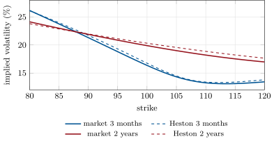
Fitted to nine strikes (80 to 120) at four expiries (three months to two years) of the surface of chapter 9, Heston returns $v_0=0.0267$ (a spot volatility of 16.3%), $\kappa=2.05$, $\bar v=0.060$ (24.5% long-run), $\eta=0.66$ and $\rho=-0.70$, with a root-mean-square error of 0.37 volatility point and at most 0.7 point, at two years (Figure 10.1). The Feller condition fails, $2\kappa\bar v-\eta^2=-0.19$: the fitted variance can touch zero, as it does in most index calibrations.

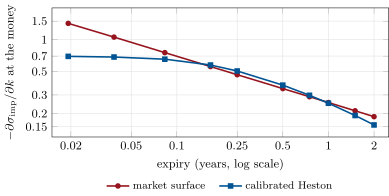
The fit hides a structural gap that shows at expiries outside the calibration set. Heston’s at-the-money skew tends to a finite limit as the expiry shrinks, while market skews keep steepening, roughly like $T^{-1/2}$ in this surface. At one week the calibrated model’s skew is half the market’s (Figure 10.2); jumps (chapter 13) and rough volatility (chapter 12) are the two answers.

10.5 What the parameters mean to a trader

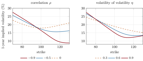
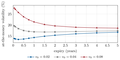
Each parameter moves one feature of the surface (Figures 10.3 and 10.4):

• $\rho$ tilts the smile: more negative, steeper skew. Moving $\rho$ from $-0.7$ to $-0.5$ lowers the one-year 90–110 skew from 5.71 to 3.94 volatility points.
• $\eta$ bends it: the wings rise with the volatility of volatility. The one-year curvature measure $\tfrac12(\sigma_{90}+\sigma_{110})-\sigma_{100}$ is 0.30 point at $\eta=0.6$; a curvature of 0.5 point needs $\eta=0.77$.
• $v_0$ and $\bar v$ set the short and long ends of the at-the-money term structure, and $\kappa$ the speed at which one becomes the other; $\kappa$ also makes the skew fade with the expiry, since variance shocks are forgotten at that rate.

For a trader the most useful identity is the one that holds without correlation.

Proposition 10.5 (Mixing formula)

If $\rho=0$, a European option in a stochastic volatility model is worth the Black–Scholes price at the path’s root-mean variance, averaged over the variance paths: $C=\E\bigl[C_{\mathrm{BS}}(\bar\sigma)\bigr]$ with $\bar\sigma^2=\frac1T\int_0^Tv_t\,dt$. With $\rho\ne0$ the same holds after replacing the spot by an adjusted spot and the variance by $(1-\rho^2)$ times it; this is the mixing formula.

The formula explains the smile’s shape at once: Black–Scholes prices are convex in volatility away from the money, so averaging over random volatility raises out-of-the-money prices more than at-the-money ones, and the smile curves up (the volga of chapter 4 at work). A simulation of variance paths with $\rho=0$ gives, through the formula, 7.136 for the one-year at-the-money call against 7.137 from the characteristic function, well within its standard error of 0.011.

10.6 Tutorial: pricing and calibrating Heston

10.7 Build: the Heston model

10.8 Exercises

Exercise 10.1 ★

Check the Feller condition for the base parameters and for the calibrated ones.

Solution

Solution of Exercise 10.1.

Base: $2\times1.5\times0.04-0.6^2=-0.24$; calibrated: $2\times2.05\times0.060-0.66^2=-0.19$. Both fail: the variance can reach zero, which the characteristic function handles, but a naive simulation must truncate.

Exercise 10.2 ★

With $v_0=0.08$, $\bar v=0.04$ and $\kappa=1.5$, give the deterministic variance after six months and one year, and the at-the-money volatility of a one-year option as $\eta\to0$.

Solution

Solution of Exercise 10.2.

$v(t)=\bar v+(v_0-\bar v)e^{-\kappa t}$: 0.0589 at six months, 0.0489 at one year. The one-year total variance is $0.04+0.04(1-e^{-1.5})/1.5=0.0607$: a volatility of 24.6%.

Exercise 10.3 ★

Why must $\varphi_{x_T}(-i)=1$? What would a value of 1.01 mean?

Solution

Solution of Exercise 10.3.

$\varphi(-i)=\E[e^{x_T}]=\E[S_T]/F=1$ because the forward is the expectation of $S_T$ under the pricing measure. A value of 1.01 means the model’s forward is 1% off: every call is mispriced by about 1% of the forward, an arbitrage against the futures market, usually a sign of a wrong branch or a coding error.

Exercise 10.4 ★★

Why does the market price of volatility risk not appear in the calibrated model, and what does that imply about using historical volatility to set $\bar v$?

Solution

Solution of Exercise 10.4.

Under the pricing measure the drift of the variance already contains it: calibration to options estimates $\kappa\bar v$ and $\kappa$ as they are priced, not as they behave. Historical volatility estimates the real-world level, which is typically below the priced one (the variance risk premium of chapter 14); setting $\bar v$ from history underprices options.

Exercise 10.5 ★★

Use the mixing formula to explain why, with $\rho=0$, the Heston smile is symmetric in log-moneyness around the forward and why its at-the-money volatility lies below the root-mean variance.

Solution

Solution of Exercise 10.5.

With $\rho=0$ the price is an average of Black–Scholes prices with the forward fixed; in log-moneyness the Black–Scholes implied volatility of such an average is symmetric around $k=0$ (put and call at $\pm k$ correspond by put–call symmetry). Near the money the Black–Scholes price is nearly linear in volatility, so the average price corresponds to the average volatility $\E[\bar\sigma]$, which is below $\sqrt{\E[\bar\sigma^2]}$ by Jensen’s inequality.

Exercise 10.6 ★★

Which parameter would you move to fit a market in which the one-month skew steepened overnight while the one-year skew did not? Why can Heston not fit it with one parameter move?

Solution

Solution of Exercise 10.6.

The short skew is steered by $\rho$ and $\eta$, the long skew too, and $\kappa$ controls how fast the skew decays with expiry: steepening only the short end needs a higher $\kappa$ and a larger $\eta$ at once, which also changes the curvature and the term structure. Heston’s skew term structure has a fixed shape, and a local event in one part of it cannot be fitted by moving one parameter.

Exercise 10.7 ★★★

Coding. With eta_for_butterfly, find the volatility of volatility that gives a one-year curvature of 0.5 volatility point, and the one-year 90–110 skew at that $\eta$.

Solution

Solution of Exercise 10.7.

$\eta=0.77$; the one-year 90–110 skew rises to 6.45 points, since with a negative correlation the volatility of volatility also steepens the skew.

Exercise 10.8 ★★★

Find the flaw. “Our Heston calibration fits the three-month to two-year surface within 0.4 points, so we use it to price weekly options on the index.”

Solution

Solution of Exercise 10.8.

The model was calibrated where it fits; at one week its skew is half the market’s, so it underprices short out-of-the-money puts and gives the wrong hedges there. Price weeklies from the market’s own short-dated smile, or with a model that produces steep short skews (jumps, rough volatility).

10.9 Problem: Reading the Parameters

Problem 10.1

Weekend problem — what each Heston number does to the smile

A junior trader inherits the base Heston model ($v_0=\bar v=0.04$, $\kappa=1.5$, $\eta=0.6$, $\rho=-0.7$, zero rates) and must adjust it to two changes in the market: the one-year 90–110 skew falls by about 1.8 points, and the one-year curvature rises to 0.5 point.

Part I — The base smile.

1. Give the one-year implied volatilities at the 80, 90, 100, 110 and 120 strikes.
2. Give the one-year 90–110 skew and the curvature measure.
3. Is the Feller condition satisfied?
4. Why is the at-the-money volatility below 20% although $v_0=\bar v=0.04$?
5. What does the model predict for the at-the-money volatility at five years?

Part II — The correlation.

6. Give the 90–110 skew with $\rho=-0.5$.
7. Give the change in skew for the change of 0.2 in correlation.
8. Does the at-the-money volatility move when $\rho$ changes? Why?
9. Which products are most exposed to $\rho$?
10. What does $\rho=-0.7$ say about the index when it falls 1% in a day?

Part III — The volatility of volatility.

11. Give the $\eta$ that produces a one-year curvature of 0.5 point.
12. What happens to the skew at that $\eta$, and why?
13. How would you restore the skew?
14. What is the Feller gap at that $\eta$?
15. Which products are most exposed to $\eta$?

Part IV — Judgement.

16. Why should the trader recalibrate all five parameters rather than move one at a time?
17. Why might the desk keep $\kappa$ fixed across days?
18. What does the model get wrong at one week?
19. State the named result: the change in the one-year 90–110 skew for a change of $+0.2$ in the correlation, and the volatility of volatility that matches a curvature of 0.5 point.
20. In one sentence: what does the volatility of volatility price?

Solution

Solution of Problem 10.1.

1. 23.4%, 20.1%, 16.9%, 14.4%, 13.3%. 2. Skew 5.71 points; curvature 0.30 point. 3. No: $2\kappa\bar v-\eta^2=-0.24$. 4. Averaging over random variance lowers the average volatility (Jensen), and the negative correlation lowers the at-the-money volatility further: 16.9% at one year. 5. 17.4%, still below 20% for the same reason. 6. 3.94 points. 7. $-1.77$ points. 8. A little: the correlation shifts probability between the tails and the forward is fixed, so the at-the-money price changes by a second-order amount. 9. Risk reversals, and every product whose value depends on the skew: barriers, digitals, autocallables. 10. That volatility tends to rise when the index falls. A 1% fall is a shock $dW^1=-0.01/\sqrt{v}=-0.05$; since $d\sqrt v\approx\tfrac12\eta\,dW^2$ and $\E[dW^2\mid dW^1]=\rho\,dW^1$, the expected rise of $\sqrt v$ is $\tfrac12\times0.6\times0.7\times0.05=0.0105$: about one volatility point. 11. $\eta=0.77$. 12. It steepens to 6.45 points: with a negative correlation the volatility of volatility adds skew as well as curvature. 13. Make the correlation less negative until the skew is back at its target. 14. $2\times1.5\times0.04-0.77^2=-0.47$. 15. Wing options, variance swaps’ convexity (chapter 14), cliquets and volatility-of-volatility products. 16. Parameters interact (here $\eta$ moves the skew too); moving them one at a time leaves the others wrong. 17. $\kappa$ and $\eta$ are nearly redundant for a surface up to a few years; fixing $\kappa$ removes a flat direction of the fit and makes the other parameters stable day to day (chapter 24). 18. Its skew levels off where the market’s keeps steepening: half the market’s at one week. 19. $-1.77$ volatility points for $+0.2$ in $\rho$; $\eta=0.77$ for a curvature of 0.5 point. 20. The uncertainty of future variance, which raises the price of options whose value is convex in volatility: the wings.

10.10 Interview questions

Interview question 10.1 ★ trader, researcher

Write the Heston model and say what each parameter does to the smile.

Solution

Solution of Interview question 10.1.

$dS=\sqrt vS\,dW^1$, $dv=\kappa(\bar v-v)dt+\eta\sqrt v\,dW^2$, $d\langle W^1,W^2\rangle=\rho\,dt$. $v_0$: short-dated level; $\bar v$: long-dated level; $\kappa$: how fast one becomes the other, and how fast the skew fades; $\eta$: the smile’s curvature (wings); $\rho$: its skew.

What the interviewer is looking for: one sentence per parameter, on the surface.

Interview question 10.2 ★ researcher

Why is a stochastic volatility market incomplete, and how do you hedge an option in it?

Solution

Solution of Interview question 10.2.

Two Brownian motions, one traded risky asset: the variance risk cannot be hedged with the share. Hedge the delta with the share and the vega (variance exposure) with another option, typically of the same expiry; the second option makes the market complete in the model.

What the interviewer is looking for: the count of risks against instruments.

Interview question 10.3 ★★ researcher

Derive the price of a European option in a stochastic volatility model with zero correlation.

Solution

Solution of Interview question 10.3.

Condition on the whole variance path: with zero correlation $\ln S_T$ is normal with variance $\int v\,dt$, so the conditional price is Black–Scholes at that variance; average over variance paths (the mixing formula).

What the interviewer is looking for: conditioning and independence.

Interview question 10.4 ★★ developer, researcher

Your Heston pricer returns wrong prices for long expiries with a large volatility of volatility. What do you suspect?

Solution

Solution of Interview question 10.4.

The complex logarithm in the characteristic function jumping branches (the “little Heston trap”): use the form with $g=(\xi-d)/(\xi+d)$ and $e^{-dT}$, which stays on the principal branch; also check the integration range and the damping of the Fourier integral.

What the interviewer is looking for: branch cuts, then numerics.

Interview question 10.5 ★★ trader, risk

Your calibrated Heston correlation moved from $-0.7$ to $-0.4$ overnight with the same fit error. What do you do?

Solution

Solution of Interview question 10.5.

Check the inputs first (a bad quote, a stale expiry); then check whether the fit has a flat direction ($\rho$ and $\eta$ trading off); stabilise the calibration (fix $\kappa$, penalise parameter changes, chapter 24) and measure the P&L effect of the jump on exotics before accepting it; if the market really moved, the exotics’ reserves should reflect it.

What the interviewer is looking for: data, identifiability, stability, P&L impact.

Interview question 10.6 ★★★ researcher

Why is the Heston skew too flat at short expiries? Name two ways to fix it.

Solution

Solution of Interview question 10.6.

Its short-dated smile comes only from the diffusion of variance over a short time, so the at-the-money skew tends to a constant proportional to $\rho\eta/\sqrt{v_0}$ as the expiry shrinks, while the market’s grows. Fixes: add jumps (chapter 13), which produce skew at short expiries, or make volatility rough (chapter 12), which produces a skew exploding like a power of the expiry.

What the interviewer is looking for: the short-expiry limit, and the two families of fixes.