Derivatives and Volatility · Derivatives
14Variance Swaps and Volatility Derivatives
A variance swap has no strike in price. Its only strike is a volatility, squared, and it pays the difference between that number and the variance the index actually realises. It looks like a bet that needs a model of volatility. It needs none. Its hedge is a fixed strip of every out-of-the-money option on the index, each weighted by one over its strike squared, plus a position in the index that is rebalanced every day. The volatility index is that strip’s price, quoted as a volatility. This chapter builds the replication, the index formula and its errors, and the convexity that separates a swap on volatility from a swap on variance. It then covers futures and options on the volatility index, and the jumps and truncated strikes that break the replication.
14.1 Variance swaps and their replication
Definition 14.1 (Variance swap)
A variance swap is a forward contract on realised variance. At expiry the long side receives , where is the annualised realised variance of daily closes, with no mean subtracted, and is the strike, quoted as a volatility.
Definition 14.2 (Variance notional)
The variance notional is the payment per unit of variance (per “variance point” when variance is quoted in percent squared).
Definition 14.3 (Vega notional)
The vega notional of a variance swap is : the approximate payment for one volatility point of realised volatility above the strike, near the strike. Trades are quoted in vega notional and settled in variance notional.
The payoff is convex in realised volatility. With a vega notional of 100 000 per point and a strike of 22.1%, the variance notional is per variance point. A realised volatility of 30% pays rather than the 790 000 a linear payoff would give, and 15% costs 596 000 rather than 710 000. The long side gains more than proportionally when volatility spikes. That convexity is why a variance swap is replicable and a volatility swap is not.
Proposition 14.4 (Replication)
If the index moves continuously, with any volatility process, then
and, with the forward and zero rates,
Realised variance is therefore the payoff of a static strip of out-of-the-money options with weights , a forward, and a dynamic position of in the index. The fair strike is
Proof. Itô’s formula (One Quant Book 4, chapter 3) for gives ; integrate and rearrange. For the second identity, any twice differentiable payoff satisfies (Taylor’s formula with integral remainder), and has . The dynamic leg has zero price, and so has the forward, which leaves the strip. ∎
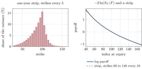
The proof never used a model for . That is the product’s appeal: the strike is read from option prices alone. The dealer who sells the swap buys the strip once, trades the index every day and is hedged, whatever volatility does, as long as the index does not jump. The strip’s weights also say what the strike is made of (Figure 14.1). On chapter 9’s surface the one-year strike is 22.1%, against an at-the-money volatility of 19.2%. Puts carry 72% of the variance, strikes below 80 carry 24%, and strikes above 120 carry 1.5%. A variance swap on a skewed index is largely a position in its downside.
A variance swap is marked to market by splitting it in time. After a time with realised variance , the expected final variance is the time-weighted average of the realised part and the fair strike of the remaining part. The value is times the discounted difference from . A one-year swap struck at 22.1% that has realised 25% over six months, with six-month variance-swap volatility at 20.1%, expects variance points against a strike of 488.4. On a variance notional of 2 262 it is worth 59 000.
14.2 The log contract and the volatility-index formula
Definition 14.5 (Log contract)
The log contract pays at . Its price, with zero rates, is the variance-swap strike in another unit. It is not listed, and is traded as its option strip.
The volatility index turns the strip into a published number. On a listed option chain the integral becomes a sum over strikes, and the index formula is
with the mid-quote of the out-of-the-money option at , the strike at or just below the forward, and half the distance between neighbouring strikes. The last term corrects for using the put and call at rather than at . Between and the strip holds an in-the-money call as an out-of-the-money put, and the term removes the difference to second order. Two expiries that bracket thirty days are computed and interpolated to a constant thirty days.
As of September 2026 — The volatility index’s methodology
Cboe’s methodology document for the index (version 6.0, last revised 26 February 2026) specifies the formula above. It uses S&P 500 options at mid-quote, keeps only options with a non-zero bid, brackets thirty days with two expiries, standard or weekly, and states the formula’s basis as the 1999 research note of Demeterfi, Derman, Kamal and Zou. A filtering algorithm guards against quotes that widen suddenly. Futures and options on the index settle on a special opening quotation that follows slightly different rules from the spot index.
How good is the sum? It has two errors: the spacing between strikes, and the range the strikes cover, which in the index is cut wherever bids vanish. On chapter 9’s thirty-day smile, whose exact strip volatility is 16.30%, the index-style number errs as in Table 14.1. Wide spacing biases it up, since a coarse sum over a convex function overstates it. A short range biases it down, since the missing wings would have added variance. A strip that stops at 95 misses 1.6 to 1.8 points. The two errors can cancel by accident, as the strip from 90 in steps of 2.5 shows.
| lowest strike (highest lowest) | |||
|---|---|---|---|
| 70 | |||
| 80 | |||
| 85 | |||
| 90 | |||
| 95 |
14.3 Volatility swaps and convexity
Definition 14.6 (Volatility swap)
A volatility swap pays : realised volatility, not variance, against a strike.
The payoff is linear in volatility, which is what many clients want to trade, but volatility is the square root of variance and no static strip replicates a square root of a path integral. Its fair strike is , and Jensen’s inequality puts it below the variance-swap strike . A second-order expansion of the square root around the mean variance gives
so the convexity adjustment is proportional to the variance of realised variance: it needs a model for the volatility of volatility. It is the convexity adjustment of One Quant Book 2, chapter 8, applied to a square root.
In Heston’s model it is exact. The Laplace transform of integrated variance, , has the closed form of an affine model. The identity turns it into by one integral. The build does exactly that, and its tests check it against a simulation.
Example 14.7 (Volatility or variance)
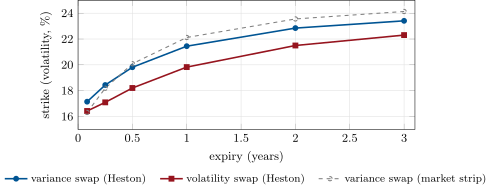
Under the Heston model calibrated to chapter 9’s surface in chapter 10, the one-year variance-swap strike is 21.4% and the volatility-swap strike 19.8%: a convexity adjustment of 1.62 volatility points. The adjustment is 0.72 point at one month, 1.34 at three months and 1.61 at six months, then falls to 1.35 at two years and 1.10 at three (Figure 14.2). At short expiries there is little time for variance to vary. At long expiries mean reversion averages its variation away. The market’s own one-year strip gives 22.1%, 0.7 point above Heston’s, because the calibrated model does not reproduce the surface’s wings, which carry weight in the strip.
Variance can be weighted and restricted, and two variants are traded. Each is replicated by the same argument with a different function of the price.
Definition 14.8 (Gamma swap)
A gamma swap pays realised variance weighted by the index level relative to its initial value, , against a strike. It is replicated by the payoff , whose second derivative is : its strip weights puts less than the variance swap’s.
Definition 14.9 (Corridor variance swap)
A corridor variance swap accrues realised variance only on days when the index is inside a range . Its strip keeps the weights on strikes in only.
The gamma swap’s variance does not explode when the index falls, since each day’s variance is multiplied by , which is small after a crash. That makes it a much less dangerous product to be short than the variance swap. On chapter 9’s surface its one-year strike is 20.8%, between the at-the-money 19.2% and the variance swap’s 22.1%. A down-corridor () isolates the variance paid in falling markets, the part of the variance swap that the skew makes expensive.
14.4 Futures and options on the volatility index
Futures on the volatility index have traded since March 2004 and options since February 2006. Chapter 12 showed that the index is, idealised, the square root of the average forward variance over thirty days, and that its future is . The future therefore lies below the forward variance-swap volatility by a convexity gap. The gap is the same Jensen effect as the volatility swap’s, applied to thirty days of variance seen from .
Example 14.10 (The futures curve under Heston)
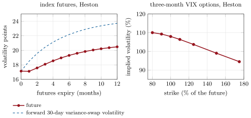
Under the calibrated Heston model the index is 17.1 today. The three-month future is 18.1 against a forward thirty-day variance-swap volatility of 20.4, the six-month 19.3 against 22.2, and the one-year 20.5 against 23.7 (Figure 14.3, left). The model computes the futures exactly: is affine in , whose Laplace transform is known, so the same square-root identity applies. A desk that reads the forward volatility off the futures curve without the gap overstates the futures’ fair level by one to three points.
Definition 14.11 (VIX option)
A VIX option is a European option on the volatility index at its expiry. It is cash-settled, and its natural underlying is the VIX future of the same expiry, so it is quoted with Black’s formula on the future.
A VIX option is an option on the forward-variance curve, so its smile measures the distribution of future volatility. The market’s VIX smile slopes upward: calls on high volatility are expensive. Baldeaux and Badran point to this observed upward skew. Under the calibrated Heston model the three-month smile slopes the other way, from 110% at 80% of the future to 94% at 175% (Figure 14.3, right). The square-root process has a thin right tail. Rough Bergomi’s VIX smile is nearly flat (chapter 12). Fitting the VIX smile’s slope with the same model as the index smile is the joint calibration problem of chapter 12.
Definition 14.12 (Variance risk premium)
The variance risk premium is the difference between the variance-swap strike and the expected realised variance under the real-world measure, (some authors use the opposite sign). It is what the seller of variance earns on average for bearing the risk of variance spikes.
Where the premium is positive, a seller of variance swaps earns it on average and pays it back, with interest, in crashes, when realised variance exceeds the strike many times over. Its size, sign and variation across underlyings are empirical questions. Carr and Wu (2009) is the classic study of them with synthetic variance swaps, and One Quant Book 6 measures them. The distinction matters for this chapter: the replication argument gives the strike under the pricing measure, and says nothing about whether selling it pays.
14.5 Skew, jumps and the limits of replication
The replication holds if the index moves continuously. Over a day with log-return , the hedge (the strip plus the daily position ) earns while the swap’s leg pays . The difference is
negligible for ordinary days and not for crashes. A fall of 20% in log costs the hedged seller of variance per unit of notional on that one day. In a model with jumps the fair strike is therefore not the strip: . With negative jumps the correction is positive, and the strip underprices the variance swap.
Example 14.13 (The strip under Merton’s jumps)
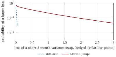
With chapter 13’s Merton model (3.16 jumps a year of mean log-size and dispersion 4.6%), each jump leaves the hedge short by of variance on average ( to leading order). The fair strike exceeds the strip’s by 0.00058 of variance a year, or 0.18 volatility point. On 100 000 three-month paths, a seller who strikes at the strip and hedges daily loses 0.17 point on average (0.18 up to simulation error), with a standard deviation of 0.40 point and a one-in-a-hundred loss of 1.9 points. In a diffusion of the same variance the same hedge has a standard deviation of 0.014 point (Figure 14.4).
Three other limits matter in practice.
- The strikes run out. The strip exists only where options are quoted. In a crash the index falls through the lowest strike, beyond which the hedge is linear while the payoff keeps growing. The truncation error in Table 14.1 then turns from a pricing bias into a loss. Martin records that the large price jumps of 2008 and 2009 disrupted volatility-derivatives markets and caused the single-name variance-swap market to dry up completely.
- Caps. A variance swap can carry a cap on realised variance, set at a multiple of the strike. The cap is a short call on variance, priced with a model of volatility of volatility, not with the strip.
- Discrete sampling and dividends. Daily closes, the absence of a mean in the estimator, and the dividend-adjusted forward all move the fair strike by small, computable amounts that the build’s mark-to-market must use consistently.
14.6 Tutorial: replicate a variance swap
Goal. Price a variance swap from a strip on a synthetic surface, compute the index-style number and its errors, value volatility swaps and index futures exactly under Heston, and simulate the hedge with and without jumps. End state: the four figures, the table and the numbers of the weekend problem.
The index formula, with , the averaged option at and the forward correction:
def index_variance(strikes, calls, puts, fwd: float, t: float, rate: float = 0.0) -> float:
    """The volatility-index formula on one expiry: (2/T) sum dK_i / K_i^2 e^(RT) Q(K_i) - (1/T)(F/K0 - 1)^2,
    with Q the put below K0, the call above, their average at K0 (K0 = the strike at or below F), and dK_i
    half the distance between the neighbouring strikes (one-sided at the ends)."""
    k = np.asarray(strikes, float)
    c, p = np.asarray(calls, float), np.asarray(puts, float)
    i0 = int(np.searchsorted(k, fwd, side="right")) - 1
    q = np.where(np.arange(len(k)) < i0, p, c)
    q[i0] = 0.5 * (c[i0] + p[i0])
    dk = np.empty_like(k)
    dk[1:-1] = 0.5 * (k[2:] - k[:-2])
    dk[0], dk[-1] = k[1] - k[0], k[-1] - k[-2]
    return float(2 / t * np.sum(dk / k ** 2 * math.exp(rate * t) * q) - (fwd / k[i0] - 1) ** 2 / t)
Listing 14.1. The volatility-index formula on one expiry. code/firm/varswap/firm_varswap.py The jump error of the log-contract hedge, one line that decides the hedge’s residual:
def jump_error(j):
    """Per-return shortfall of the log-contract hedge against the variance swap's leg: the hedge earns
    2 (e^r - 1 - r) for a log-return r and the swap pays r^2; for small r the difference is about r^3 / 3."""
    j = np.asarray(j, float)
    return 2 * (np.exp(j) - 1 - j) - j * j
Listing 14.2. Shortfall of the hedge on a return . code/firm/varswap/firm_varswap.py Heston’s volatility swap by the Laplace transform of integrated variance and the square-root identity:
def _sqrt_expectation(laplace, scale: float) -> float:
    """E[sqrt(X)] = (1 / (2 sqrt(pi))) int_0^inf (1 - E[e^(-s X)]) s^(-3/2) ds, on s = scale * e^y."""
    y = np.linspace(-25.0, 25.0, 4001)
    s = scale * np.exp(y)
    integrand = (1 - laplace(s)) * s ** -0.5          # s^(-3/2) ds = s^(-1/2) dy
    return float(np.trapezoid(integrand, y) / (2 * math.sqrt(math.pi)))


def integrated_cir_laplace(s, v0: float, kappa: float, vbar: float, eta: float, t: float):
    """E[exp(-s int_0^T v dt)] for the square-root process (the affine 'bond price' formula)."""
    s = np.asarray(s, float)
    g = np.sqrt(kappa * kappa + 2 * eta * eta * s)
    e = np.exp(-g * t)                                # written with e^(-g t) to stay finite for large s
    den = (g + kappa) * (1 - e) + 2 * g * e
    b = 2 * s * (1 - e) / den
    a = 2 * kappa * vbar / eta ** 2 * (np.log(2 * g / den) + 0.5 * (kappa - g) * t)
    return np.exp(a - b * v0)


def heston_vol_swap(v0: float, kappa: float, vbar: float, eta: float, t: float) -> float:
    """E[sqrt((1/T) int_0^T v dt)], the fair volatility-swap strike in Heston."""
    mean = heston_mean_variance(v0, kappa, vbar, t)
    return _sqrt_expectation(lambda s: integrated_cir_laplace(s / t, v0, kappa, vbar, eta, t), 1 / mean)
Listing 14.3. Exact volatility-swap strike under Heston. code/firm/varswap/firm_varswap.py - Run
dv_varswap.index_errors(),heston_terms(),vix_curve(),hedge_pnl()andfig_varswap.py.
What to change next. Replace the square-root identity by the second-order approximation and measure its error at one year; cut the strip where the model’s put price falls below 0.05 (a “zero bid”) and recompute the thirty-day number; price a down-corridor variance swap with .
14.7 Build: variance and volatility swaps
Purpose. The miniature firm’s pricer and mark-to-market for variance swaps, and the volatility-swap and index-future values that its volatility desk quotes against.
Interface. index_variance(strikes, calls, puts, fwd, t, rate); strip_from_vols; log_payoff_strip; realised_variance(prices); variance_notional(vega_notional, strike_vol); mark_to_market(var_notional, strike_vol, realised_var, t_elapsed, fair_var_remaining, t_remaining, df); jump_error(r); vol_swap_approx; heston_mean_variance, heston_vol_swap, heston_vix_future.
Rules. Strikes are quoted in volatility and settled in variance; the realised-variance estimator is the contract’s (daily closes, 252 days, no mean); the strip uses the forward, not the spot; every model value is checked against a simulation in the tests.
Acceptance tests. code/firm/varswap/tests/: a flat smile’s index number is its volatility, with the forward between strikes; the strip reproduces the log payoff inside its range; the conventions (notional conversion, mark-to-market); the jump error behaves like ; Heston’s Laplace transforms equal one at zero, the volatility swap tends to the variance swap as the volatility of volatility vanishes and matches a simulation, and index futures lie below the forward.
Stretch. Capped variance swaps under Heston; corridor and gamma swaps from a listed chain; the special opening quotation’s rules for settlement.
Sources and further reading
- K. Demeterfi, E. Derman, M. Kamal and J. Zou, “More than you ever wanted to know about volatility swaps”, Goldman Sachs Quantitative Strategies Research Notes (March 1999).
- Cboe Global Markets, “Cboe Volatility Index Methodology”, version 6.0 (2026).
- P. Carr and R. Lee, “Volatility derivatives”, Annual Review of Financial Economics 1 (2009) 319–339.
- P. Carr and L. Wu, “Variance risk premiums”, Review of Financial Studies 22(3) (2009) 1311–1341.
- I. Martin, “Simple variance swaps”, NBER Working Paper 16884 (2011).
- J. Baldeaux and A. Badran, “Consistent modeling of VIX and equity derivatives using a 3/2 plus jumps model”, arXiv 1203.5903 (2012).
14.8 Exercises
Exercise 14.1 ★
A client wants 50 000 of vega notional on a variance swap struck at 20%. What is the variance notional, and what does the swap pay if realised volatility is 25%?
Solution
Solution of Exercise 14.1.
per variance point; at 25% the swap pays .
Exercise 14.2 ★
Why does a variance swap need a daily trade in the index as well as the option strip?
Solution
Solution of Exercise 14.2.
The strip pays , which equals realised variance only after adding : the gains of holding in the index. Without the daily trade the position is a log contract, whose payoff depends on where the index ends, not on the path.
Exercise 14.3 ★
Show that the gamma swap’s replicating payoff has second derivative , and explain why its strike is below the variance swap’s on a downside-skewed index.
Solution
Solution of Exercise 14.3.
and . Its strip weights are against for the variance swap: relative to the variance swap it weights each strike by , less below the spot and more above. On a downside-skewed index the expensive puts count for less, so the strike is lower.
Exercise 14.4 ★★
After nine months a one-year variance swap struck at 22% has realised 18%, and the three-month variance-swap volatility is 16%. Value it per unit of variance notional (variance in percent squared, zero rates).
Solution
Solution of Exercise 14.4.
Expected final variance against : the value is per unit of variance notional.
Exercise 14.5 ★★
Use the second-order approximation to estimate the volatility-swap strike when the variance-swap strike is 20% and the standard deviation of realised variance is 0.02.
Solution
Solution of Exercise 14.5.
, : .
Exercise 14.6 ★★
Why does the convexity adjustment in Example 14.7 peak near one year?
Solution
Solution of Exercise 14.6.
The adjustment is proportional to the variance of realised variance divided by its level. At short expiries variance has no time to move; at long expiries mean reversion (, a half-life of about four months) averages its moves away. The variance of the average is largest when the expiry is a few half-lives long.
Exercise 14.7 ★★★
Coding. Compute the thirty-day index-style number with strikes every 1 from 80 to 120 and then drop the strikes whose out-of-the-money option is worth less than 0.05. How much does the number fall?
Solution
Solution of Exercise 14.7.
The full strip gives 16.32%; the options worth at least 0.05 run from 87 to 106, and the number falls to 16.10%, 0.22 point lower: the missing wings carried variance.
Exercise 14.8 ★★★
Find the flaw. “We sell variance swaps at the strip’s price and hold the strip and the daily delta; the book is fully hedged, so the premium we charge over the strip is pure profit.”
Solution
Solution of Exercise 14.8.
The hedge is exact only for continuous paths within the strip’s range. Each jump leaves a loss of about of variance, and a crash through the lowest strike leaves the payoff growing while the hedge stops. The premium over the strip is the price of that jump and truncation risk (0.18 point on average under chapter 13’s Merton model, with a one-in-a-hundred loss of 1.9 points over three months), not profit.
14.9 Problem: Vol or Variance
Problem 14.1
Weekend problem — the price of a square root
A client asks for one-year quotes on a variance swap and on a volatility swap on the index of chapter 9’s surface. The desk has the surface, the Heston calibration of chapter 10, and the build.
Part I — The variance swap.
- Give the one-year variance-swap strike from the strip and the at-the-money volatility.
- Which strikes carry the strike? Give the puts’ share.
- For a vega notional of 100 000, give the variance notional and the payoff at 30% realised volatility.
- What would the thirty-day index-style number lose with a strip that stops at 95?
- Give the one-year gamma-swap strike.
Part II — The volatility swap under Heston.
- Give Heston’s one-year variance-swap strike, and explain the gap to the strip’s.
- Give the one-year volatility-swap strike.
- Give the convexity adjustment at one month, one year and three years.
- Which Heston parameter drives the adjustment, and in which direction?
- Why is the volatility swap not replicable with a static strip?
Part III — The index and its options.
- Give the index level and the three-month and one-year futures under Heston.
- Give the convexity gap at three months.
- Describe the three-month VIX smile under Heston.
- How would the desk hedge a volatility swap?
- What premium over the strip would you charge a client who buys the variance swap, if the index can jump?
Part IV — Judgement.
- The client says the volatility swap “should be priced at the variance-swap strike, since both are volatility”. Answer in two sentences.
- Which model assumption does the convexity adjustment depend on most?
- What reserve would you hold on a short volatility swap hedged with variance swaps?
- State the named result: the convexity adjustment between the one-year variance-swap and volatility-swap strikes on the chapter’s surface under Heston dynamics.
- In one sentence: why is variance, not volatility, the traded quantity?
Solution
Solution of Problem 14.1.
1. 22.1% and 19.2%. 2. The puts: 72% of the variance; strikes below 80 alone 24%. 3. 2 262 per variance point; 931 000. 4. 1.6 to 1.8 points, depending on the spacing. 5. 20.8%. 6. 21.4%: the calibrated model misses the surface’s wings, which the strip weights heavily. 7. 19.8%. 8. 0.72, 1.62 and 1.10 points. 9. The volatility of variance : 1.24 points at , 2.01 at . 10. Its payoff is the square root of realised variance, a non-linear function of the path’s quadratic variation; only functions of the terminal price are static strips, and variance is the one path functional that reduces to one. 11. 17.1, 18.1 and 20.5. 12. points. 13. It slopes down, from 110% at 80% of the future to 94% at 175%. 14. With variance swaps, dynamically: a volatility swap’s sensitivity to variance is about , so the desk holds variance swaps in that ratio and adjusts it as volatility moves, a hedge whose cost is the volatility of volatility the adjustment prices. 15. At least the jump correction, 0.18 point under chapter 13’s jump model, plus a reserve for crashes through the strip. 16. Volatility is the square root of variance, and the mean of a square root is below the square root of the mean. The difference, here 1.6 points, is the price of the volatility of volatility. 17. The distribution of realised variance, above all the volatility of volatility . 18. A reserve for the model: the spread of the adjustment across plausible (about 0.4 point either way for ) and the cost of re-hedging in a volatility spike. 19. 1.62 volatility points: 21.4% against 19.8% at one year. 20. Variance is replicated by a static strip and a delta; volatility needs a model.
14.10 Interview questions
Interview question 14.1 ★ trader, researcher
How do you replicate a variance swap?
Solution
Solution of Interview question 14.1.
Itô’s formula gives . Hold a static strip of out-of-the-money options with weights (the log payoff) and trade in the underlying daily; the strike is the strip’s price per unit of time.
What the interviewer is looking for: the log contract, the weights and the dynamic leg.
Interview question 14.2 ★ trader
Why is the variance-swap strike above the at-the-money volatility on an index?
Solution
Solution of Interview question 14.2.
The strip weights options by , so low strikes count more, and on an index the low strikes trade at higher implied volatilities. The strike is an average of variance over the whole smile, tilted to the downside.
What the interviewer is looking for: the weights and the skew.
Interview question 14.3 ★★ researcher
Is a volatility swap’s fair strike above or below the variance swap’s? By how much, roughly?
Solution
Solution of Interview question 14.3.
Below, by Jensen’s inequality. To second order the gap is : about 1.6 points at one year under a Heston model calibrated to a typical index surface, more with a higher volatility of volatility.
What the interviewer is looking for: the sign, the expansion, and that it needs a model.
Interview question 14.4 ★★ developer
Implement the volatility-index formula for one expiry. What edge cases matter?
Solution
Solution of Interview question 14.4.
Find the forward from put–call parity, at or below it, take puts below and calls above (both averaged at ), weight by with one-sided differences at the ends, subtract , interpolate two expiries to thirty days. Edge cases: the forward exactly on a strike; zero bids and where to cut the wings; uneven strike spacing; stale quotes; expiry times in minutes.
What the interviewer is looking for: the formula, the correction and the data cases.
Interview question 14.5 ★★ risk, trader
What happens to a dealer short a variance swap, hedged with the strip, when the index gaps down 20%?
Solution
Solution of Interview question 14.5.
The swap’s leg pays of variance for the day while the hedge earns : a loss of about . If the gap goes below the strip’s lowest strike the hedge also stops tracking. Losses scale with notional and there is no dynamic fix; the protection is pricing the jump risk, caps, and buying deep puts.
What the interviewer is looking for: the cubic term, the strip’s range, and caps.
Interview question 14.6 ★★★ trader, risk
Why must a VIX future be priced below the forward variance-swap volatility, and how would you trade the gap?
Solution
Solution of Interview question 14.6.
The future is and the forward variance-swap volatility is ; Jensen’s inequality makes the first smaller, by an amount set by the volatility of the index. To trade it: buy the forward variance (a calendar spread of variance swaps) against a short future, which is long the volatility of the index, and hedge its vega with index options; the position profits if realised volatility of the index exceeds what the gap prices.
What the interviewer is looking for: Jensen, and what the spread is exposed to.