University Biology — Year 2 · Bachelor Year 2

27Global Change and the Biosphere

Between 1851 and 1858 Henry Thoreau walked the woods and meadows around Concord, Massachusetts, and wrote down the day each of some five hundred plants first flowered. A century and a half later, botanists went back to the same places with his notebooks. The highbush blueberry that Thoreau saw open on May 11 now opens on April 12; the whole flora flowers, on average, ten days earlier than in his time, in step with a spring that is $2.4\,{}^{\circ}\mathrm{C}$ warmer; and a quarter of his species are gone from Concord — not at random, but those whose flowering could not track the temperature. The previous chapters gave the machinery: the cycles of Chapter 25, the selection and drift of Chapter 22, the competition and speciation of Chapter 23, the soils of Chapter 26. This chapter puts a number on what is happening to living things as one species changes the chemistry of the air and the sea: how much warming per tonne of carbon, how many days of spring per degree, how many metres uphill, how much acid in the sea, how many species per hectare lost — and what the numbers say about the century ahead.

27.1 The physical change

Proposition 27.1 (Warming is proportional to cumulative emissions)

Carbon dioxide absorbs the infrared the ground emits and returns a part of it; more $\mathrm{CO_2}$ means a warmer surface, by about $3\,{}^{\circ}\mathrm{C}$ for each doubling once the oceans have caught up (the climate sensitivity). Because the temperature response to $\mathrm{CO_2}$ is logarithmic in concentration while the airborne fraction of emissions falls as the concentration rises, the two curvatures nearly cancel, and the global mean warming is, to a good approximation, linear in the cumulative amount of carbon emitted, whatever the timing:

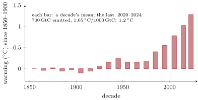
\Delta T \approx \lambda\,C_{\text{cum}}, \qquad \lambda \approx 1.65\,{}^{\circ}\mathrm{C} \text{ per } 1000\,\mathrm{GtC}

( $0.45\,{}^{\circ}\mathrm{C}$ per $1000\,\mathrm{Gt}$ of $\mathrm{CO_2}$ ). Some $700\,\mathrm{GtC}$ emitted since 1850 have warmed the planet by $1.2\,{}^{\circ}\mathrm{C}$ — and the relation gives every target a budget: $1.5\,{}^{\circ}\mathrm{C}$ allows about $900\,\mathrm{GtC}$ in all, $200\,\mathrm{GtC}$ more than has been emitted, twenty years at the present rate. The warming is unequal: twice the average over land and three times in the Arctic; nights more than days; and it comes with the rest — more intense rain and longer droughts, a sea level rising $4\,\mathrm{mm}$ a year, ice that is a fifth smaller in summer, and an ocean that has absorbed $90\,\%$ of the heat and a quarter of the carbon.

Evidence. The proportionality was found in climate models of every complexity and confirmed by the observed record: plotting the warming since 1850 against cumulative emissions gives a straight line through the decades. The greenhouse effect itself is measured from orbit: satellites see the infrared the Earth emits with the absorption bands of $\mathrm{CO_2}$ , methane and water vapour cut out of it, and the cut has deepened between 1970 and 2020 by exactly the amount the rise in these gases predicts. The isotopes and the falling oxygen of Chapter 25 tie the extra $\mathrm{CO_2}$ to fossil fuel. ∎

Global mean surface temperature by decade, relative to the second half of the nineteenth century. The last four decades each set a record, and the rise since 1970 is 0.2\, C per decade. — Global mean surface temperature by decade, relative to the second half of the nineteenth century. The last four decades each set a record, and the rise since 1970 is $0.2\,{}^{\circ}\mathrm{C}$ per decade.

27.2 The calendar: phenology

Theorem 27.2 (Degree-days and the advance of spring)

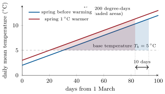
Many events in the life of plants and ectotherms — budburst, flowering, egg hatching, emergence — occur when the accumulated thermal time since a start date, the sum of daily temperatures above a base $T_b$ (degree-days), reaches a fixed total $K$ . If spring temperature rises linearly, $T(t) = T_b + b\,(t - t_0)$ at $b$ degrees per day from the day $t_0$ it crosses the base, the event occurs at

t^{*} = t_0 + \sqrt{2K/b},

and a uniform warming of $\Delta T$ brings the crossing day forward by $\Delta T/b$ and the event with it: with $b \approx 0.1\,{}^{\circ}\mathrm{C}$ per day, about ten days earlier per degree. Species differ in $T_b$ , $K$ and in whether they also use day length, which warming does not change — so the members of a food chain advance at different rates and their timing comes apart: a phenological mismatch between the caterpillar and the bird that must feed its chicks on it.

Proof. Degree-days from $t_0$ : $\int_{t_0}^{t}(T - T_b)\,\mathrm{d}t' = b\,(t - t_0)^{2}/2$ , equal to $K$ when $t - t_0 = \sqrt{2K/b}$ . Warming by $\Delta T$ replaces $T$ by $T + \Delta T$ : the base is crossed $\Delta T/b$ days earlier and the accumulation, identical from that day on, completes $\Delta T/b$ days earlier. (If the warming also steepens $b$ , the interval $\sqrt{2K/b}$ shortens too.) A species cued by day length keeps its date; one cued by degree-days moves; the gap between them grows by $\Delta T/b$ . ∎

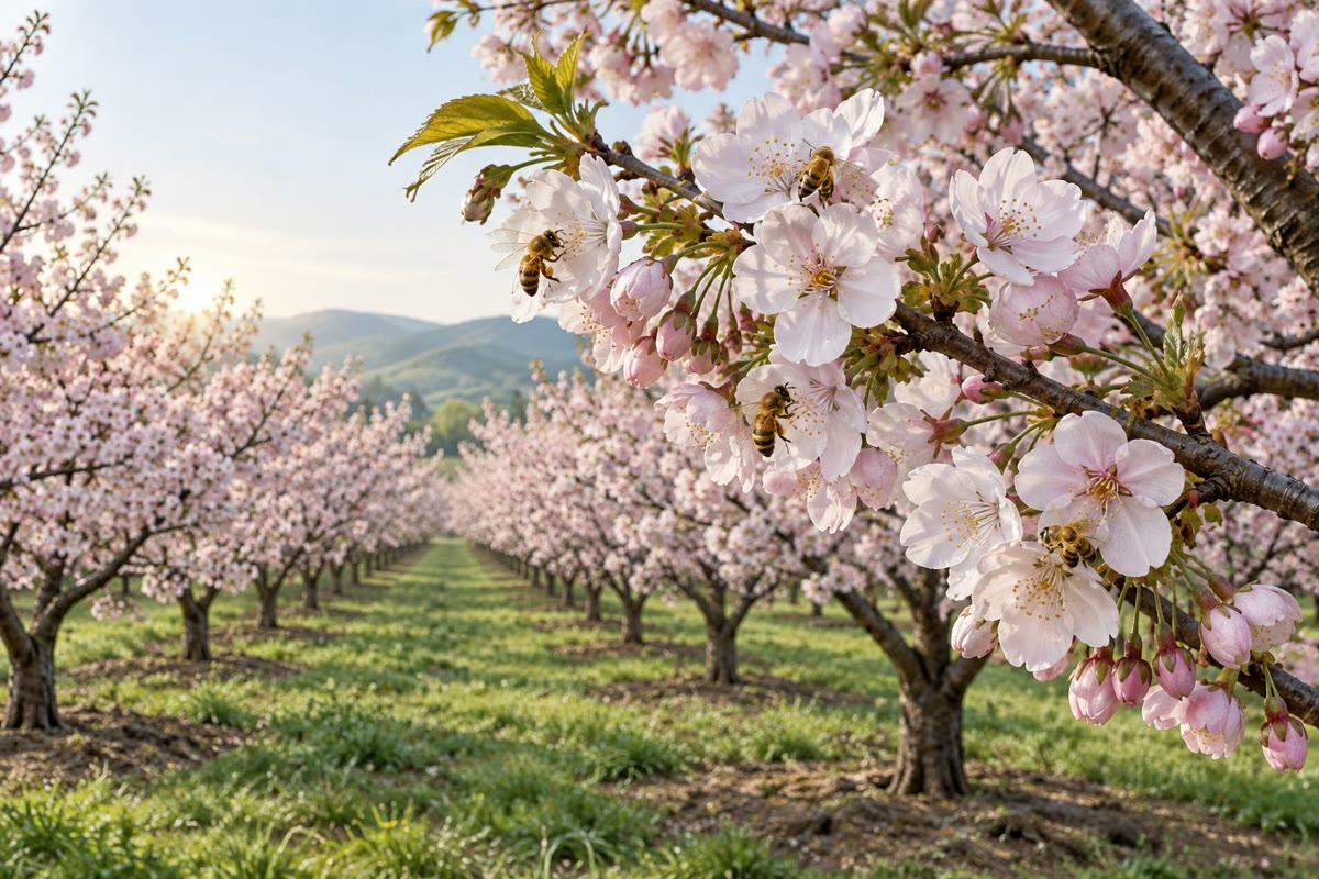
Evidence. Thoreau’s Concord flora, and the Marsham family’s record of twenty-seven signs of spring in Norfolk kept from 1736 to 1947, both show flowering and leafing advancing by $3\text{ to }6\,\mathrm{d}$ per degree of spring warming. The Kyoto cherry blossom, dated in court diaries since the ninth century, held around mid-April for a thousand years and has moved to early April since 1900, the earliest dates on record falling in the 2020s. In the Netherlands the oak’s caterpillars now peak two weeks earlier than in 1985; the great tit, cued by the same warmth, has kept pace, but the pied flycatcher, which times its migration from Africa by day length, arrives as before and finds the peak gone — its populations have fallen by $90\,\%$ where the mismatch is largest (Both and colleagues, 2006). ∎

A cherry orchard in bloom. The Kyoto cherries, dated in diaries for twelve centuries, now open earlier than in any year before 1900 — and the bees that pollinate them must be flying on the same day.

Degree-days. The event occurs when the shaded area between the temperature line and the base reaches K; a spring one degree warmer crosses the base ten days sooner and completes the sum ten days sooner. — Degree-days. The event occurs when the shaded area between the temperature line and the base reaches $K$ ; a spring one degree warmer crosses the base ten days sooner and completes the sum ten days sooner.

27.3 The map: range shifts

Proposition 27.3 (Isotherms move, and species follow)

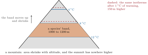
Temperature falls by about $6.5\,{}^{\circ}\mathrm{C}$ per kilometre of altitude and by about $0.65\,{}^{\circ}\mathrm{C}$ per hundred kilometres of latitude in the temperate zone; a warming of $1\,{}^{\circ}\mathrm{C}$ therefore moves every isotherm about $150\,\mathrm{m}$ uphill and $150\,\mathrm{km}$ poleward. Species whose limits are set by temperature move with their isotherm if they can: the average of hundreds of studied species has shifted $11\,\mathrm{m}$ uphill and $17\,\mathrm{km}$ poleward per decade since 1970, at the speed of the isotherms, and the fastest — mobile, generalist, short-lived — outrun them, while trees, whose seeds travel metres a year, and species already at the summit or the pole, cannot follow: a mountain’s top has nowhere to go, and each degree of warming removes the highest $150\,\mathrm{m}$ of every range. Marine species, with no barriers and sharper thermal limits, move fastest, tens of kilometres a decade; the cod, the mackerel and the fisheries with them have moved north across whole seas. The upper edge of a range advances, the lower edge retreats as it warms and as new competitors arrive from below, and the community at any point is reassembled from species that have never met.

Evidence. Parmesan (1996) resurveyed the Edith’s checkerspot butterfly across its western North American range: populations at the southern edge and low altitudes were extinct, those at the northern edge and high altitudes thriving, and the whole range had moved $92\,\mathrm{km}$ north and $124\,\mathrm{m}$ up — the first species shown to have tracked the isotherms. Lenoir and colleagues (2008) compared forest plant surveys of 1905–1985 with 1986–2005 across the French mountains: the optimum altitude of 171 species had risen by $29\,\mathrm{m}$ a decade. Chen and colleagues (2011), across two thousand species, found the shifts two to three times faster than earlier estimates, and proportional to the local warming. ∎

A range shift on a mountain. Each degree lifts the isotherms 150\, m; a species tracks its band upward into a smaller area, and a band already at the summit is lost. — A range shift on a mountain. Each degree lifts the isotherms $150\,\mathrm{m}$ ; a species tracks its band upward into a smaller area, and a band already at the summit is lost.

27.4 The sea: acidification and heat

Theorem 27.4 (Acidification)

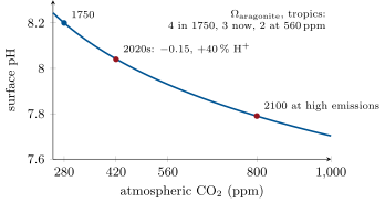
Carbon dioxide dissolving in seawater makes carbonic acid, which dissociates: ${\mathrm{CO_2}} + {\mathrm{H_2O}} \rightleftharpoons {\mathrm{H^{+}}} + {\mathrm{HCO_3^{-}}}$ , with $[{\mathrm{H^{+}}}][{\mathrm{HCO_3^{-}}}]/[{\mathrm{CO_2}}] = K_1$ . Bicarbonate is the ocean’s largest carbon pool and is held nearly constant by the alkalinity, so

[{\mathrm{H^{+}}}] \propto p_{{\mathrm{CO_2}}}, \qquad \Delta\mathrm{pH} \approx -\log_{10}\frac{p_{{\mathrm{CO_2}}}}{p_0}

— more precisely $-0.9\log_{10}$ of the ratio, because bicarbonate rises a little. From 280 to $420\,\mathrm{ppm}$ the surface pH has fallen by $0.15$ , from $8.2$ to $8.05$ : a $40\,\%$ increase in hydrogen ions; at $800\,\mathrm{ppm}$ it would fall by $0.4$ . The extra hydrogen ions consume carbonate, ${\mathrm{H^{+}}} + {\mathrm{CO_3^{2-}}} \to {\mathrm{HCO_3^{-}}}$ , and the saturation state $\Omega$ of calcium carbonate — the product of calcium and carbonate concentrations over the solubility product — falls in proportion: shells and skeletons of aragonite (corals, pteropods) form readily at $\Omega > 3$ , with difficulty near 1, and dissolve below it; the tropical surface, at $\Omega \approx 4$ before industry and 3 now, reaches 2 at $560\,\mathrm{ppm}$ , and the cold, $\mathrm{CO_2}$ -rich polar surface waters reach 1 first.

Proof. From the equilibrium, $[{\mathrm{H^{+}}}] = K_1[{\mathrm{CO_2}}]/[{\mathrm{HCO_3^{-}}}]$ and $[{\mathrm{CO_2}}]$ is proportional to $p_{{\mathrm{CO_2}}}$ by Henry’s law; with $[{\mathrm{HCO_3^{-}}}]$ constant, $[{\mathrm{H^{+}}}]$ is proportional to $p_{{\mathrm{CO_2}}}$ and $\mathrm{pH} = -\log_{10}[{\mathrm{H^{+}}}]$ changes by $-\log_{10}$ of the ratio. The second equilibrium, $[{\mathrm{H^{+}}}][{\mathrm{CO_3^{2-}}}]/[{\mathrm{HCO_3^{-}}}] = K_2$ , gives $[{\mathrm{CO_3^{2-}}}] \propto 1/[{\mathrm{H^{+}}}] \propto 1/p_{{\mathrm{CO_2}}}$ , so $\Omega$ falls as $p_{{\mathrm{CO_2}}}$ rises, and the $40\,\%$ rise in $[{\mathrm{H^{+}}}]$ is a $30\,\%$ fall in carbonate. (The full chemistry, with the change in bicarbonate and the ion activities, gives the factor $0.9$ and the observed numbers; the Year 3 volume treats it.) ∎

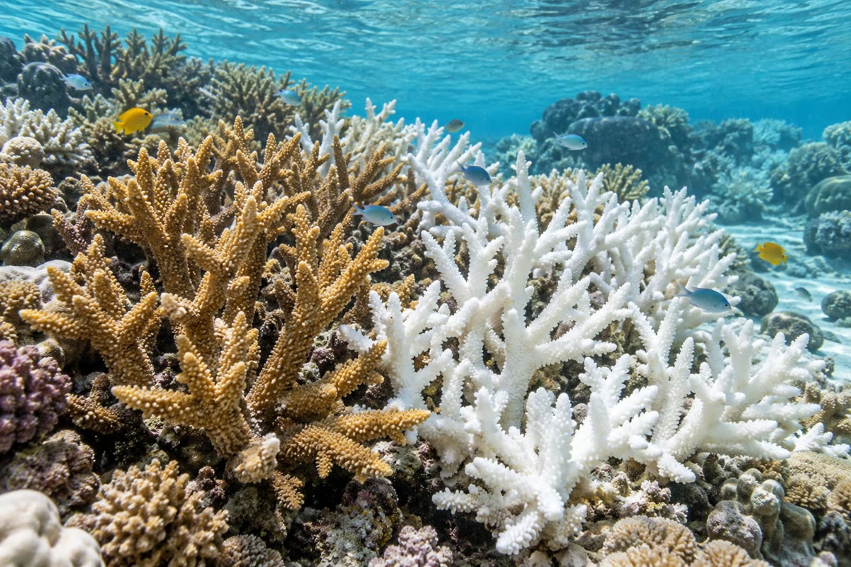
Evidence. The ocean station north of Hawaii has measured surface pH monthly since 1988: it falls by $0.0018$ a year, in step with the $\mathrm{CO_2}$ at Mauna Loa above it, as the chemistry requires. Pteropods — the sea’s snails, food for salmon and whales — collected off the Pacific coast show their aragonite shells pitted and dissolving where upwelling brings water with $\Omega < 1$ to the surface. Coral bleaching is heat, not acid: when the water stays $1\,{}^{\circ}\mathrm{C}$ above the summer maximum for a few weeks, the coral expels its symbiotic algae and starves; the Great Barrier Reef bleached in 1998, 2002, 2016, 2017, 2020, 2022 and 2024, and half its coral cover is gone since 1995. ∎

Surface ocean pH against atmospheric carbon dioxide, pH = 8.2 - 0.9 _10(p/280). The scale is logarithmic: each tenth of a unit is a quarter more hydrogen ions. — Surface ocean pH against atmospheric carbon dioxide, $\mathrm{pH} = 8.2 - 0.9\log_{10}(p/280)$ . The scale is logarithmic: each tenth of a unit is a quarter more hydrogen ions.

Two thermometers. Left: a bleached reef, the coral’s white skeleton showing through tissue that has lost its algae. Right: a valley glacier that has withdrawn up its valley, leaving bare rock where ice stood a century ago.

27.5 The ledger: extinction and its estimate

Theorem 27.5 (The species–area relation and the cost of habitat loss)

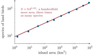
The number of species found in an area $A$ grows as a power of the area, $S = cA^{z}$ , with $z \approx 0.25$ for islands and habitat fragments (doubling the area adds a fifth more species; a hundredfold more area, three times as many). If a habitat is reduced to a fraction $1 - h$ of its extent, the number of species it can eventually hold falls to $(1 - h)^{z}$ of the original: a loss of half the habitat costs $16\,\%$ of its species, $90\,\%$ costs $44\,\%$ , and $99\,\%$ costs $68\,\%$ . The loss is not immediate — the survivors in the fragment persist for a while, an extinction debt paid over decades as small populations succumb to the drift and inbreeding of Chapter 22 — and it is the basis of the estimate that the current extinction rate is a hundred to a thousand times the background rate of the fossil record: about one species in a million per year, against the several thousand a year, out of some ten million, now being lost.

Proof. $S'/S = (A'/A)^{z} = (1 - h)^{z}$ ; with $z = 0.25$ , $0.5^{0.25} = 0.84$ , $0.1^{0.25} = 0.56$ , $0.01^{0.25} = 0.32$ . The relation itself is empirical; its exponent reflects the balance, on islands, between the immigration of new species (falling as the island fills) and the extinction of resident ones (rising as their populations shrink with area), the equilibrium of MacArthur and Wilson’s theory. ∎

Evidence. The islands of the Krakatau group, sterilised by the eruption of 1883, were recolonised by plants, birds and insects in a succession that reached, within fifty years, the species numbers predicted from their areas; the mangrove islets Simberloff and Wilson fumigated in Florida in 1966 returned to their original species counts, with different species, within a year. The Atlantic forest of Brazil, reduced to $10\,\%$ of its extent, has lost or nearly lost the fraction of its bird species the relation predicts; and in every group assessed by the World Conservation Union, a quarter to a third of species are threatened — birds $13\,\%$ , mammals $27\,\%$ , amphibians $41\,\%$ , corals $44\,\%$ — with habitat loss the first cause, and hunting, invasive species, pollution and, increasingly, climate the others. ∎

The species–area relation, here for land birds on islands of an archipelago: a straight line of slope z = 0.25 on logarithmic axes. Cut a habitat to a tenth and it will, in time, keep little more than half of its species. — The species–area relation, here for land birds on islands of an archipelago: a straight line of slope $z = 0.25$ on logarithmic axes. Cut a habitat to a tenth and it will, in time, keep little more than half of its species.

Proposition 27.6 (Invasions, services, and what can be done)

Ships, planes and trade have moved thousands of species past the barriers that kept them apart; most fail to establish, but the few that do — the rabbit in Australia, the zebra mussel in the Great Lakes, the brown tree snake that emptied Guam of its birds, the chytrid fungus that has driven ninety amphibian species to extinction — spread as a front advancing at constant speed, $c = 2\sqrt{rD}$ for a population growing at rate $r$ and dispersing with diffusion coefficient $D$ (Skellam’s muskrat, released near Prague in 1905, expanded across Europe at $11\,\mathrm{km}$ a year, its range radius a straight line in time). Against all this stands what the biosphere does for its one troublesome species: pollination of three quarters of crops, water purification, flood control, the fixing of nitrogen and the making of soil, fisheries, the carbon held in forests and soils — ecosystem services valued, where a price can be put on them, at more than the world’s economic product. What can be done follows from the numbers. Warming stops when net emissions do, and not before: the box models of Chapter 25 allow no other reading of net zero. Land can help within limits — a gigatonne of carbon a year from reforestation and soils for a few decades, against ten from fossil fuels — and species can be helped to move, or kept in reserves large and connected enough that the species–area relation and the drift of small populations do not finish them. The tools are those of this book: the population genetics of the reserve, the competition of the invader, the phenology of the crop, the budget of the soil.

Example 27.7 (Three futures)

Emissions held at $10\,\mathrm{GtC}$ a year to 2100 add $800\,\mathrm{GtC}$ to the $700\,$ already emitted: $1.65\times 1.5 = 2.5\,{}^{\circ}\mathrm{C}$ by the century’s end and still rising. Emissions falling to zero by 2070 add about $250\,\mathrm{GtC}$ : $1.6\,{}^{\circ}\mathrm{C}$ , then level. Doubling emissions first, as the century’s early decades did, gives $4\,{}^{\circ}\mathrm{C}$ or more. The ranges of the temperate zone move $200\,\mathrm{km}$ beyond today’s in the first case and $60\,\mathrm{km}$ in the second; spring comes twenty-five days earlier, or six; surface pH reaches $7.8$ , or stays near $8.0$ ; and the extinction estimates, which depend on habitat and warming together, range from a tenth to a third of species. The difference between the futures is the cumulative area under one curve, which is the sum of decisions not yet made.

27.6 Exercises

Exercise 27.1 ★

State the relation between warming and cumulative emissions, and compute the warming for cumulative emissions of 700, 1000 and $2000\,\mathrm{GtC}$ .

Solution

Solution of Exercise 27.1.

$\Delta T = \lambda C_{\text{cum}}$ with $\lambda = 1.65\,{}^{\circ}\mathrm{C}$ per $1000\,\mathrm{GtC}$ : $1.2\,{}^{\circ}\mathrm{C}$ , $1.65\,{}^{\circ}\mathrm{C}$ , $3.3\,{}^{\circ}\mathrm{C}$ .

Exercise 27.2 ★

Define degree-days and phenological mismatch, with the flycatcher as an example.

Solution

Solution of Exercise 27.2.

Degree-days: the sum over days of the excess of the daily mean temperature over a base, the thermal time that governs the development of plants and ectotherms. Mismatch: when two interacting species time their seasons by different cues and warming moves one and not the other — the flycatcher, cued by day length in Africa, arrives on its old date to find the caterpillar peak, cued by temperature, already two weeks past.

Exercise 27.3 ★

How far do isotherms move uphill and poleward per degree of warming, and why can a mountain-top species not follow?

Solution

Solution of Exercise 27.3.

About $150\,\mathrm{m}$ uphill and $150\,\mathrm{km}$ poleward per degree. A species at the summit has no higher ground: its isotherm rises above the mountain and its habitat disappears, while the area of each band shrinks with altitude on the way up.

Exercise 27.4 ★

Explain in three sentences why adding $\mathrm{CO_2}$ to the sea lowers its pH and its carbonate, and which organisms are hurt.

Solution

Solution of Exercise 27.4.

Dissolved $\mathrm{CO_2}$ forms carbonic acid, which releases hydrogen ions, and the pH falls in proportion to the logarithm of the $\mathrm{CO_2}$ pressure. The extra hydrogen ions convert carbonate to bicarbonate, so the carbonate concentration and the saturation state of calcium carbonate fall. Organisms that build aragonite — corals, pteropods, many larvae — and calcite — coccolithophores, foraminifera, molluscs — must spend more to build shells and, below saturation, lose them.

Exercise 27.5 ★★

Compute the carbon budget remaining for $1.5\,{}^{\circ}\mathrm{C}$ and for $2\,{}^{\circ}\mathrm{C}$ with $\lambda = 1.65\,{}^{\circ}\mathrm{C}$ per $1000\,\mathrm{GtC}$ and $700\,\mathrm{GtC}$ already emitted; convert both to years at $10\,\mathrm{GtC}/\mathrm{yr}$ .

Solution

Solution of Exercise 27.5.

$1.5\,{}^{\circ}\mathrm{C}$ : $1.5/1.65\times 1000 = 909\,\mathrm{GtC}$ in all, $209\,\mathrm{GtC}$ remaining, 21 years. $2\,{}^{\circ}\mathrm{C}$ : $1212\,\mathrm{GtC}$ , $512\,\mathrm{GtC}$ remaining, 51 years.

Exercise 27.6 ★★

Spring warms at $b = 0.12\,{}^{\circ}\mathrm{C}$ per day from a base of $5\,{}^{\circ}\mathrm{C}$ ; a moth needs $K = 150$ degree-days. Compute the days from base-crossing to emergence, and the advance for a warming of $1.5\,{}^{\circ}\mathrm{C}$ .

Solution

Solution of Exercise 27.6.

$\sqrt{2\times 150/0.12} = 50$ days; advance $1.5/0.12 = 12.5$ days.

Exercise 27.7 ★★

A plant’s range spans $800\text{ to }1400\,\mathrm{m}$ on a mountain $1800\,\mathrm{m}$ high whose area halves every $300\,\mathrm{m}$ of altitude. After $3\,{}^{\circ}\mathrm{C}$ of warming, where is the band and how much area has it lost? After $5\,{}^{\circ}\mathrm{C}$ ?

Solution

Solution of Exercise 27.7.

$3\,{}^{\circ}\mathrm{C}$ : isotherms rise $3000/6.5 = 460\,\mathrm{m}$ ; the band moves to $1260\text{ to }1860\,\mathrm{m}$ , but the mountain ends at $1800\,\mathrm{m}$ : the top $60\,\mathrm{m}$ of the band are lost and the rest sits where the area is $2^{-460/300} = 0.35$ of what it was — about two thirds of the area gone. $5\,{}^{\circ}\mathrm{C}$ : $770\,\mathrm{m}$ ; the band would be $1570\text{ to }2170\,\mathrm{m}$ ; only $1570\text{ to }1800\,\mathrm{m}$ exists, a third of the band’s width at $2^{-770/300} = 0.17$ of the area — under a tenth of the original area: the species is effectively gone.

Exercise 27.8 ★★

Compute the surface pH and the rise in hydrogen-ion concentration at 560, 800 and $1000\,\mathrm{ppm}$ , from $\mathrm{pH} = 8.2 - 0.9\log_{10}(p/280)$ .

Solution

Solution of Exercise 27.8.

560: pH $7.93$ , hydrogen ions $\times 1.9$ ; 800: $7.79$ , $\times 2.6$ ; 1000: $7.70$ , $\times 3.1$ .

Exercise 27.9 ★★

With $z = 0.25$ , what fraction of species is eventually lost when $70\,\%$ , $95\,\%$ and $99.9\,\%$ of a habitat is destroyed? Why is the immediate loss smaller?

Solution

Solution of Exercise 27.9.

$1 - (1 - h)^{0.25}$ : $26\,\%$ , $53\,\%$ , $82\,\%$ . The immediate loss is smaller because the remnant still holds populations of most species; they are too small to persist and die out over decades — the extinction debt.

Exercise 27.10 ★★★

An invader grows at $r = 0.7$ per year and disperses with $D = 20\,\mathrm{km}^{2}/\mathrm{yr}$ . Compute its front speed and the time to cross a country $1000\,\mathrm{km}$ wide. What halves the speed: halving $r$ or halving $D$ ?

Solution

Solution of Exercise 27.10.

$c = 2\sqrt{0.7\times 20} = 7.5\,\mathrm{km}/\mathrm{yr}$ ; $1000\,\mathrm{km}$ in about 130 years. Halving either $r$ or $D$ divides $c$ by $\sqrt 2$ , to $5.3\,\mathrm{km}/\mathrm{yr}$ ; neither halves it — to halve the speed one must quarter the product $rD$ .

Exercise 27.11 ★★★

The background extinction rate is 1 per million species-years and there are 8 million species. Compute the expected extinctions a year and per century at background, and at 1000 times background. Compare with the ten thousand documented extinctions of the last century and comment on the discrepancy.

Solution

Solution of Exercise 27.11.

Background: $8\times 10^{6}\times 10^{-6} = 8$ a year, 800 a century; at a thousand times, 8000 a year, $800\,000$ a century. Ten thousand documented in a century is about ten times background, not a thousand — but documentation covers only the few per cent of species that are described and monitored (birds, mammals, a few plants), among which the rate is indeed a hundred times background or more; for the undescribed majority, most extinctions are never seen, and the species–area estimate is the only handle. The truth lies between the counted and the estimated, which is why the range quoted is so wide.

Exercise 27.12 ★★★

“Warming stops when net emissions stop.” Justify from the box model of the atmosphere and the proportionality of warming to cumulative emissions, and say what is missing from the argument.

Solution

Solution of Exercise 27.12.

The temperature is proportional to cumulative emissions; when net emissions are zero the cumulative total stops growing and so does the warming. In the box model, with emissions zero, the atmospheric excess begins to fall as the sinks work on, which would cool — but the ocean, still warming toward equilibrium with the raised $\mathrm{CO_2}$ , continues to warm the surface, and the two effects nearly cancel: the temperature stays where it is for centuries. Missing from the argument: the other greenhouse gases (methane’s short lifetime means its warming falls quickly once emissions stop), the aerosols that now mask some warming and vanish within weeks of the emissions that make them, and the feedbacks — permafrost carbon, forest dieback — that could add emissions of their own.

27.7 Problem: The Biosphere in 2100

Problem 27.1

Weekend problem — two emission paths carried to 2100: the warming of each, the spring it makes, the distance its isotherms travel, the acid it puts in the sea and the species it costs a forest, ending on the two warmings, the two pH values and the fraction of species lost

Data. $\lambda = 1.65\,{}^{\circ}\mathrm{C}$ per $1000\,\mathrm{GtC}$ ; $700\,\mathrm{GtC}$ emitted by 2020 (warming $1.2\,{}^{\circ}\mathrm{C}$ ). Path A: $10\,\mathrm{GtC}/\mathrm{yr}$ constant to 2100. Path B: falling linearly to zero in 2070. Spring warms at $b = 0.1\,{}^{\circ}\mathrm{C}$ per day above a base of $5\,{}^{\circ}\mathrm{C}$ ; a tree needs $K = 200$ degree-days to leaf, and a migratory bird arrives on a fixed date, 20 days after the tree’s leafing in 2020. Lapse rate $6.5\,{}^{\circ}\mathrm{C}/\mathrm{km}$ ; latitudinal gradient $0.65\,{}^{\circ}\mathrm{C}$ per $100\,\mathrm{km}$ . Ocean: $\mathrm{pH} = 8.2 - 0.9\log_{10}(p/280)$ ; $\mathrm{CO_2}$ in 2100: $600\,\mathrm{ppm}$ on path A, $420\,\mathrm{ppm}$ on path B. A forest region of $10^{5}\,\mathrm{km}^{2}$ with 400 tree species, $z = 0.25$ , loses $60\,\%$ of its area to clearing by 2100 on path A and $20\,\%$ on path B.

Part I — Warming.

Compute the cumulative emissions in 2100 on each path.
Compute the warming in 2100 on each path.
Compute the warming in 2050 on each.
What is the warming rate per decade on path A? Compare with the observed $0.2\,{}^{\circ}\mathrm{C}$ per decade.
On path B, does the warming stop in 2070? Why, according to the proportionality?
What cumulative emission corresponds to $2\,{}^{\circ}\mathrm{C}$ , and in what year does path A cross it?

Part II — Spring.

Compute the days from base-crossing to leafing in 2020.
Compute the advance of leafing, relative to 2020, in 2100 on each path (warming relative to 2020).
The bird’s arrival date does not change. Compute the gap between leafing and arrival on each path in 2100.
The caterpillars the bird needs peak 15 days after leafing and last 10 days. On which path does the bird still find them?
Suppose instead the bird advances by $3\,\mathrm{d}$ per degree. Recompute the gap on path A.
State in one sentence why the mismatch, not the warming itself, is what threatens the bird.

Part III — Ranges.

Compute the altitudinal and latitudinal displacement of isotherms on each path, relative to 2020.
A tree species disperses $100\,\mathrm{m}$ a year. Can it track the isotherms poleward on path A? On path B?
A species occupies $1500\text{ to }1800\,\mathrm{m}$ on a $2000\,\mathrm{m}$ mountain. On path A, where does its band sit in 2100, and what happens?
The mountain’s area halves every $300\,\mathrm{m}$ . Compute the area factor lost by that species on path B.
A marine fish tracks isotherms at $30\,\mathrm{km}$ a decade. Is that enough on path A?
Explain why the lower edge of a range retreats even where the species could tolerate the heat.

Part IV — Sea and forest.

Compute the surface pH in 2100 on each path, and the rise in hydrogen-ion concentration since 1750.
The saturation state $\Omega$ of the tropical surface was 4 in 1750 and falls as $[{\mathrm{H^{+}}}]^{-1}$ . Compute it in 2100 on each path and say what it means for coral.
Compute the number of tree species the forest region can eventually hold on each path, and the number lost.
Warming adds losses: suppose each degree above 2020 removes a further $5\,\%$ of the surviving species. Recompute the species remaining on each path.
Give the fraction of the 400 species lost on each path.
Which of the two causes, clearing or warming, dominates on each path?
State the result: the warming, the pH and the fraction of tree species lost in 2100 on each path.

Solution

Solution of Problem 27.1.

1. A: $700 + 80\times 10 = 1500\,\mathrm{GtC}$ . B: $700 + \tfrac12\times 50\times 10 = 950\,\mathrm{GtC}$ . 2. A: $1.65\times 1.5 = 2.5\,{}^{\circ}\mathrm{C}$ . B: $1.65\times 0.95 = 1.6\,{}^{\circ}\mathrm{C}$ . 3. 2050. A: $1000\,\mathrm{GtC}$ , $1.65\,{}^{\circ}\mathrm{C}$ . B: emissions $10\int_0^{30}(1 - t/50)\,\mathrm{d}t = 10(30 - 9) = 210\,\mathrm{GtC}$ , total 910, $1.5\,{}^{\circ}\mathrm{C}$ . 4. $\lambda\times 100 = 0.165\,{}^{\circ}\mathrm{C}$ per decade, slightly below the observed $0.2$ (which includes the other gases and the loss of aerosol masking). 5. Yes: cumulative emissions stop growing in 2070, and so does the warming, which stays at $1.6\,{}^{\circ}\mathrm{C}$ — the proportionality means the temperature is set by the total, not by the rate. 6. $2/1.65\times 1000 = 1212\,\mathrm{GtC}$ ; path A reaches it after $512/10 = 51$ years, in 2071. 7. $\sqrt{2\times 200/0.1} = 63$ days. 8. Warming relative to 2020: A $2.5 - 1.2 = 1.3\,{}^{\circ}\mathrm{C}$ , B $0.4\,{}^{\circ}\mathrm{C}$ . Advance $\Delta T/b$ : A 13 days, B 4 days. 9. Gap: A $20 + 13 = 33$ days; B 24 days. 10. Caterpillars available from day 15 to day 25 after leafing. B: the bird arrives at day 24, within the window, just. A: day 33, eight days after the last caterpillar. 11. The bird advances $3\times 1.3 = 4$ days: gap $33 - 4 = 29$ days — still outside the window. 12. The bird can live at the new temperature; what it cannot do is feed chicks when the food has gone, because its cue and its prey’s cue respond to warming differently. 13. A: $1.3/6.5\times 1000 = 200\,\mathrm{m}$ up and $1.3/0.65\times 100 = 200\,\mathrm{km}$ poleward. B: $57\,\mathrm{m}$ and $57\,\mathrm{km}$ . 14. In 80 years the tree moves $8\,\mathrm{km}$ : it cannot track $200\,\mathrm{km}$ (A) and falls short of $57\,\mathrm{km}$ (B) too — trees lag, and their ranges will be out of equilibrium with climate for centuries on either path. 15. A: the band would be $1700\text{ to }2000\,\mathrm{m}$ : it just reaches the summit, with nowhere further to go. The mountain narrows with height, so the same slice covers only $2^{-200/300} = 0.63$ times its former area — and any further warming has no ground left to move it to. 16. B: $57\,\mathrm{m}$ up, area factor $2^{-57/300} = 0.88$ : a $12\,\%$ loss. 17. Eight decades at $30\,\mathrm{km}$ : $240\,\mathrm{km}$ , more than the $200\,\mathrm{km}$ required on A: the fish keeps up (and moves out of its old fishery). 18. At the lower edge the species meets competitors, pathogens and predators moving up from below that it did not face before, and its own physiology, adapted to the old temperature, is outperformed by theirs: the retreat is competitive as much as physiological. 19. A: $\mathrm{pH} = 8.2 - 0.9\log_{10}(600/280) = 7.90$ ; hydrogen ions $10^{0.30} = 2.0$ times 1750’s. B: $8.04$ ; $1.44$ times. 20. $\Omega = 4/(\text{ratio})$ : A $2.0$ , B $2.8$ . At 2 the corals still calcify but slowly, their skeletons weaker and their reefs eroding faster than they grow; at $2.8$ they build, though the heat of path B still bleaches them. 21. A: $400\times 0.4^{0.25} = 318$ , 82 lost. B: $400\times 0.8^{0.25} = 378$ , 22 lost. 22. A: $318\times(1 - 0.05\times 1.3) = 298$ . B: $378\times(1 - 0.05\times 0.4) = 371$ . 23. A: $1 - 298/400 = 26\,\%$ . B: $7\,\%$ . 24. On both, clearing: 82 against 20 species on A, 22 against 7 on B — the model’s warming term is modest; in reality the two interact, since a fragmented forest cannot shift its range. 25. Path A: $2.5\,{}^{\circ}\mathrm{C}$ , pH $7.90$ , a quarter of the tree species lost. Path B: $1.6\,{}^{\circ}\mathrm{C}$ , pH $8.04$ , $7\,\%$ lost.