University Biology — Year 2 · Bachelor Year 2

22Population Genetics and Natural Selection

In 1848 a black peppered moth was caught near Manchester; by 1895 nineteen moths in twenty in the city were black, and by 1970, as the soot went, the pale form was back. The moths did not change: the proportions of two alleles in a population of millions did, under the eyes of birds, in a few dozen generations. Darwin had seen that selection must change species but had no way to count it; the counting is population genetics, and it is the arithmetic of this chapter. It asks how allele frequencies behave when nothing acts on them, and then how fast selection, mutation, migration, chance and inbreeding move them — and it ends with the characters that are not one gene but many, which is most of what selection actually sees.

22.1 The gene pool at rest

Definition 22.1 (Population, gene pool, frequencies)

A population is a group of individuals of one species that interbreed; its gene pool is the set of all their alleles. For a locus with two alleles $A$ and $a$ in a diploid population of $N$ individuals, the allele frequencies are $p = (2N_{AA} + N_{Aa})/2N$ and $q = 1 - p$ , and the genotype frequencies are the fractions of $AA$ , $Aa$ and $aa$ . Evolution, in the narrowest sense, is a change of allele frequencies between generations; the question of this chapter is what changes them and by how much.

Theorem 22.2 (Hardy–Weinberg)

In a large population mating at random, without selection, mutation or migration, the allele frequencies do not change from one generation to the next, and after a single generation of random mating the genotype frequencies are

AA : p^{2}, \qquad Aa : 2pq, \qquad aa : q^{2},

and stay so. Dominance does not make a dominant allele spread, and a rare recessive allele is not lost: it hides in heterozygotes, which outnumber the homozygotes $2p/q$ to one — for $q = 0.01$ , two hundred to one. The law is the null hypothesis of population genetics: a departure from it in a real population, or a change of $p$ between generations, is the signature of one of the forces below.

Proof. Random mating is random union of gametes: a gamete carries $A$ with probability $p$ and $a$ with probability $q$ , independently of its partner, so the zygote is $AA$ with probability $p^{2}$ , $Aa$ with $2pq$ , $aa$ with $q^{2}$ . The allele frequency in the next generation is $p' = p^{2} + \tfrac12(2pq) = p(p + q) = p$ : unchanged. Since the genotype frequencies depend only on $p$ , they are the same in every generation after the first. ∎

Example 22.3 (Reading a frequency)

Cystic fibrosis, recessive, affects one European child in 2500: $q^{2} = 1/2500$ , $q = 0.02$ , and the carrier frequency is $2pq \approx 0.04$ — one person in 25 carries an allele that kills its homozygotes, and $98\,\%$ of the copies of the allele sit in healthy carriers where selection cannot see them. That is why a lethal recessive is removed so slowly, and why eugenic schemes to eliminate recessive diseases by sterilising the affected never could have worked: the arithmetic of the next section shows how slowly.

22.2 Selection

Definition 22.4 (Fitness)

The fitness $w$ of a genotype is its relative contribution of offspring to the next generation — survival to reproduction times fecundity, scaled so that the best genotype has $w = 1$ . The selection coefficient $s$ of a genotype is its shortfall, $w = 1 - s$ . Fitness is a property of a genotype in an environment, not of an allele in itself: the melanic moth’s allele had $w > 1$ relative to the pale one on sooty bark and $w < 1$ on lichen.

Theorem 22.5 (Selection changes allele frequency)

With genotype fitnesses $w_{AA}$ , $w_{Aa}$ , $w_{aa}$ , the mean fitness is $\bar w = p^{2}w_{AA} + 2pq\,w_{Aa} + q^{2}w_{aa}$ and the allele frequency in the next generation is

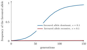
p' = \frac{p^{2}w_{AA} + pq\,w_{Aa}}{\bar w}, \qquad \Delta p = p' - p = \frac{pq\,\bigl[p(w_{AA} - w_{Aa}) + q(w_{Aa} - w_{aa})\bigr]}{\bar w}.

Two consequences. First, $\Delta p$ is proportional to $pq$ : selection is fastest at intermediate frequencies and slowest when an allele is rare or nearly fixed — there is little variation to act on. Second, against a recessive allele ( $w_{AA} = w_{Aa} = 1$ , $w_{aa} = 1 - s$ ) the change is $\Delta q = -s\,pq^{2}/\bar w$ , proportional to $q^{2}$ : a rare recessive is almost invisible to selection, and halving its frequency from $0.01$ takes about a hundred generations even when its homozygotes are lethal. A favourable dominant allele spreads fast at first and then stalls at the end, for the same reason.

Proof. Of the offspring, a fraction $p^{2}w_{AA}/\bar w$ are $AA$ and $2pq\,w_{Aa}/\bar w$ are $Aa$ (each genotype’s frequency weighted by its fitness and renormalised); the $A$ alleles among them are all of the first and half of the second, giving $p'$ . Subtracting $p = p\bar w/\bar w$ and expanding $\bar w$ gives $\Delta p$ . For a lethal recessive ( $s = 1$ ): $q' = q^{2}\cdot 0 + pq$ over $\bar w = 1 - q^{2}$ , so $q' = q/(1 + q)$ , hence $1/q' = 1/q + 1$ and after $t$ generations $1/q_t = 1/q_0 + t$ : from $q_0 = 0.01$ to $0.005$ takes $t = 100$ . ∎

Selection at work with a 10\,\% advantage. A favoured dominant allele rises from 1\,\% to a majority in seventy generations and then slows, its rare recessive rival hiding in heterozygotes; a favoured recessive allele at 1\,\% barely moves in the same time, since it is almost never exposed. — Selection at work with a $10\,\%$ advantage. A favoured dominant allele rises from $1\,\%$ to a majority in seventy generations and then slows, its rare recessive rival hiding in heterozygotes; a favoured recessive allele at $1\,\%$ barely moves in the same time, since it is almost never exposed.

Proposition 22.6 (Kinds of selection)

Directional selection favours one extreme and drives an allele toward fixation (the melanic moth in a sooty wood; antibiotic resistance; the size of a finch’s beak in a drought). Stabilising selection favours the middle and removes the extremes (human birth weight: the babies who die are the smallest and the largest); it keeps a population where it is and is the commonest kind. Disruptive selection favours both extremes against the middle, and can split a population (Chapter 23). Balancing selection keeps two alleles in the population indefinitely: by heterozygote advantage, when $Aa$ is fitter than either homozygote — with $w_{AA} = 1 - s$ , $w_{aa} = 1 - t$ , $w_{Aa} = 1$ , the frequency settles at $\hat p = t/(s + t)$ — or by frequency-dependent selection, when a genotype is fitter the rarer it is (the rare $S$ alleles of Chapter 6, prey a predator has not learned, the two mouth-sides of a scale-eating fish).

Evidence. Sickle-cell haemoglobin kills most homozygotes before they reproduce, yet the allele is at $10\,\%$ to $20\,\%$ across malarial Africa. Allison (1954) showed that heterozygous children had far fewer and milder malarial infections than either homozygote, and the allele’s frequency maps onto the historical distribution of falciparum malaria; in populations of African descent living where there is no malaria the frequency has been falling ever since. With $t \approx 0.8$ for the sickle homozygote and $s \approx 0.1$ for the normal homozygote in a malarial region, $\hat q = s/(s + t) \approx 0.11$ — what is observed. ∎

22.3 Mutation, migration, and the balance

Theorem 22.7 (Mutation–selection balance)

A deleterious allele is fed by mutation at rate $\mu$ per gamete per generation and removed by selection. At equilibrium the two balance: for a recessive allele with homozygous disadvantage $s$ ,

\hat q = \sqrt{\mu/s}\,;

for a dominant (or partly dominant) allele with heterozygous disadvantage $hs$ , $\hat q = \mu/hs$ . The equilibrium frequency of a recessive is thus large even for a lethal: with $\mu = 10^{-5}$ and $s = 1$ , $\hat q = 3\times 10^{-3}$ , and $0.6\,\%$ of the population carry it. Every population carries such a genetic load at thousands of loci, most of it recessive and hidden, and the equilibrium of Chapter 7’s ratchet argument — a fraction $e^{-U/s}$ of individuals free of deleterious mutations — is the same balance summed over the genome.

Proof. Each generation mutation adds $\mu p \approx \mu$ to $q$ and selection removes $s\,pq^{2}/\bar w \approx sq^{2}$ (for small $q$ ); setting $\mu = s\hat q^{2}$ gives the recessive result. For a dominant allele selection removes $hs\,q$ per generation (each copy is exposed in a heterozygote), and $\mu = hs\hat q$ . ∎

Proposition 22.8 (Migration and the one-migrant rule)

If a fraction $m$ of a population each generation are immigrants from a population with allele frequency $p_{m}$ , the frequency moves toward $p_{m}$ by $\Delta p = m(p_{m} - p)$ : the difference between the two populations decays as $(1 - m)^{t}$ . Gene flow homogenises; it undoes local adaptation unless selection is stronger than $m$ , and it is the force that keeps a species one species. Conversely, populations exchanging no migrants diverge by drift and by their separate mutations, and a single migrant per generation — whatever the population size — is enough to prevent them from drifting to fixation for different alleles.

22.4 Chance: genetic drift

Theorem 22.9 (Genetic drift)

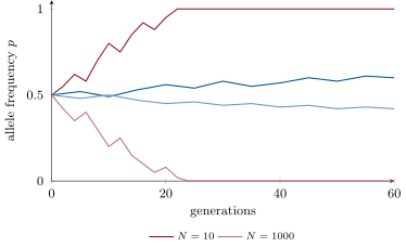
In a population of $N$ diploid individuals, each generation’s allele frequency is a random sample of $2N$ gametes from the previous one, so that $p$ wanders at random with a variance of $p(1 - p)/2N$ per generation. The heterozygosity $H = 2pq$ decays on average by a factor $(1 - 1/2N)$ each generation,

H_t = H_0\left(1 - \frac{1}{2N}\right)^{t} \approx H_0\,e^{-t/2N},

and every allele is eventually lost or fixed, with probability equal to its current frequency: a new neutral mutation, at frequency $1/2N$ , is fixed with probability $1/2N$ and, if it is, takes about $4N$ generations to do so. Drift is negligible in a population of millions and dominant in one of dozens: a bottleneck or a founder event — a few colonists on an island, a species reduced to a hundred by hunting — loses alleles by chance in a generation and leaves a population that is uniform, impoverished and full of homozygotes. The $N$ that matters is the effective size, the number of individuals actually breeding, usually much smaller than the census.

Proof. The next generation’s $2N$ gene copies are drawn with replacement from a pool in which $A$ has frequency $p$ : the number of $A$ copies is binomial with mean $2Np$ and variance $2Np(1 - p)$ , so $p'$ has mean $p$ and variance $p(1 - p)/2N$ . Two copies drawn at random in the next generation come from the same parental copy with probability $1/2N$ and are then identical, so the chance that two copies differ (the heterozygosity) is multiplied by $1 - 1/2N$ each generation. Fixation probability: a neutral allele’s frequency is a martingale — its expected value never changes — and it ends at 0 or 1, so the probability of ending at 1 equals its starting value. ∎

Drift. Two populations of ten individuals starting at p = 0.5 fix opposite alleles within twenty-five generations; two of a thousand wander by a few percent in sixty. — Drift. Two populations of ten individuals starting at $p = 0.5$ fix opposite alleles within twenty-five generations; two of a thousand wander by a few percent in sixty.

Proposition 22.10 (Inbreeding)

Mating between relatives does not change allele frequencies but raises the proportion of homozygotes: an individual’s inbreeding coefficient $F$ is the probability that its two alleles at a locus are identical by descent, and the genotype frequencies become $p^{2} + Fpq$ , $2pq(1 - F)$ , $q^{2} + Fpq$ . For the offspring of first cousins $F = 1/16$ , of siblings $1/4$ , of self-fertilisation $1/2$ . Since the recessive alleles of the genetic load are exposed in the extra homozygotes, inbred offspring suffer inbreeding depression: a lethal recessive at $q = 0.01$ appears in $q^{2} = 10^{-4}$ of random-mating offspring but in $q^{2} + Fpq = 7\times 10^{-4}$ of cousins’ children, sevenfold more; summed over thousands of loci, the children of cousins have about twice the infant mortality of others, and a small population that inbreeds for generations loses fertility and vigour — the plight of the cheetah, the Florida panther and the royal houses of Europe.

22.5 Many genes: quantitative characters

Theorem 22.11 (Heritability and the response to selection)

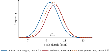
A character such as height, yield or beak depth is set by many genes of small effect and by the environment, and varies continuously. Its variance in a population splits into a genetic part $V_G$ and an environmental part $V_E$ , and the heritability $h^{2} = V_A/V_P$ is the fraction of the phenotypic variance due to the additive effects of genes (the part that is transmitted). If the parents of the next generation are selected with a mean that exceeds the population’s by $S$ (the selection differential), their offspring exceed it by

R = h^{2}\,S

— the breeder’s equation. It is the whole of animal and plant breeding in one line: a heritability of $0.5$ and parents a standard deviation above the mean give offspring half a standard deviation above it, and the gain accumulates generation after generation. Heritability is a property of a population in an environment, not of a character: it says nothing about whether a trait is fixed, and a trait with $h^{2} = 0.8$ in one population may have $h^{2} = 0$ in another where every individual has the same genotype.

Proof. The offspring’s expected phenotype regresses on the mid-parent’s with slope $h^{2}$ (the additive genetic covariance between relatives over the phenotypic variance), so a parental deviation $S$ gives an offspring deviation $h^{2}S$ . In practice $h^{2}$ is measured from that regression, or from the resemblance of twins and siblings, or from the response itself. ∎

Evidence. The Illinois maize experiment, begun in 1896, selected the ears with the highest and lowest oil content every year: after a hundred generations the high line had risen from $5\,\%$ to $20\,\%$ oil and the low line fallen to under $1\,\%$ , both still responding — the variation of many genes is not exhausted by a century of selection. In the Galápagos, the Grants measured every finch on one island through the drought of 1977: the survivors had beaks $4\,\%$ deeper than the dead, the character had $h^{2} \approx 0.7$ , and the next year’s chicks had beaks $3\,\%$ deeper than the previous generation’s — selection observed, measured, and its response predicted by the equation above. ∎

The breeder’s equation in a finch population. The drought left survivors with a mean beak S = 0.5\, mm deeper; with h2 = 0.7 their offspring were R = 0.35\, mm deeper than the generation before. — The breeder’s equation in a finch population. The drought left survivors with a mean beak $S = 0.5\,\mathrm{mm}$ deeper; with $h^{2} = 0.7$ their offspring were $R = 0.35\,\mathrm{mm}$ deeper than the generation before.

Example 22.12 (The moth’s arithmetic)

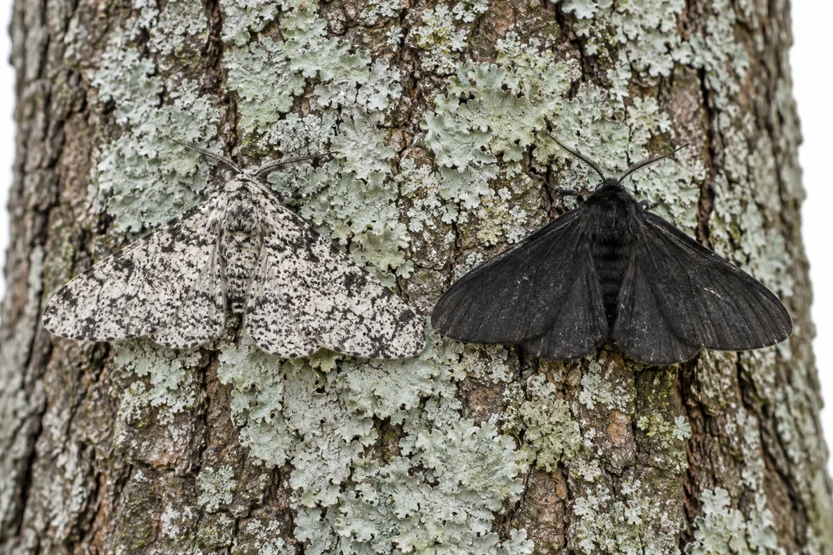
The melanic allele of the peppered moth is dominant. From a frequency of about $10^{-3}$ in 1848 to $90\,\%$ of moths (a frequency near $0.7$ ) by 1895 is fifty generations; the selection equation reproduces it with $s$ between $0.2$ and $0.3$ against the pale form — and Kettlewell’s release experiments of the 1950s, in which birds took pale moths from sooty trunks and dark ones from clean trunks in about that ratio, measured the coefficient directly. The return after clean-air laws, from $90\,\%$ melanic in 1960 to under $10\,\%$ by 2000, ran at the same speed the other way. The whole episode — a large population, a dominant allele, a strong and reversible selective agent — is population genetics happening in public.

Left: the two forms of the peppered moth on lichen — which one a bird finds depends on the bark. Right: the shell polymorphism of the grove snail, colours and bands kept in every population by predators that learn the common form.

22.6 Exercises

Exercise 22.1 ★

In a sample of 1000 people, 640 are $MM$ , 320 $MN$ and 40 $NN$ . Compute the allele frequencies and the Hardy–Weinberg expectations. Is the population in equilibrium?

Solution

Solution of Exercise 22.1.

$p(M) = (1280 + 320)/2000 = 0.8$ , $q(N) = 0.2$ . Expected $MM$ : $0.64\times 1000 = 640$ ; $MN$ : $2\times 0.8\times 0.2\times 1000 = 320$ ; $NN$ : 40 — exactly the observed numbers. The population is in equilibrium at this locus.

Exercise 22.2 ★

Albinism is recessive and affects one person in $20\,000$ . Compute the allele frequency and the carrier frequency.

Solution

Solution of Exercise 22.2.

$q = \sqrt{1/20000} = 0.0071$ ; carriers $2pq \approx 0.014$ , one person in 70. Carriers outnumber affected people by $2p/q \approx 280$ to one.

Exercise 22.3 ★

Define fitness, selection coefficient and heritability, and give the five forces that change allele frequencies.

Solution

Solution of Exercise 22.3.

Fitness: the expected number of offspring of a genotype relative to the best. Selection coefficient $s$ : the fitness deficit, $w = 1 - s$ . Heritability $h^{2}$ : the fraction of the phenotypic variance that is additive genetic, equivalently the slope of offspring on parents. Forces: mutation, selection, drift, migration, non-random mating (the last changes genotype, not allele, frequencies).

Exercise 22.4 ★

Give one example each of directional, stabilising and balancing selection, with the agent of selection in each.

Solution

Solution of Exercise 22.4.

Directional: melanism in the peppered moth, agent the birds hunting by sight on soot-darkened trunks. Stabilising: human birth weight, agent the mortality of very small and very large babies. Balancing: sickle cell, agents malaria (against $AA$ ) and anaemia (against $SS$ ) together.

Exercise 22.5 ★★

A lethal recessive allele has frequency $0.02$ . How many generations to halve it? To reach $0.001$ ? What does this say about the effect of preventing affected individuals from reproducing?

Solution

Solution of Exercise 22.5.

$q_t = q_0/(1 + tq_0)$ : halving takes $1/q_0 = 50$ generations; reaching $0.001$ takes $1/0.001 - 1/0.02 = 950$ generations. Almost all copies of the allele sit in heterozygotes, invisible to selection; preventing the affected from reproducing (which nature already does, since they are dead) changes nothing measurable in a human lifetime.

Exercise 22.6 ★★

With $w_{AA} = 1$ , $w_{Aa} = 1$ , $w_{aa} = 0.8$ and $p = 0.3$ , compute $\bar w$ , $p'$ and $\Delta p$ . Repeat for $p = 0.9$ . Why is the second change so much smaller?

Solution

Solution of Exercise 22.6.

$p = 0.3$ : $\bar w = 0.09 + 0.42 + 0.8\times 0.49 = 0.902$ ; $p' = (0.09 + 0.21)/0.902 = 0.333$ ; $\Delta p = +0.033$ . $p = 0.9$ : $\bar w = 0.998$ , $p' = 0.9018$ , $\Delta p = +0.0018$ . At $p = 0.9$ only $q^{2} = 0.01$ of the population is $aa$ : the allele selection acts against is hidden in heterozygotes, and $\Delta p = spq^{2}/\bar w$ carries the factor $q^{2}$ .

Exercise 22.7 ★★

The sickle-cell homozygote has $w = 0.2$ and the normal homozygote $w = 0.88$ in a malarial region, heterozygotes $w = 1$ . Compute the equilibrium frequency of the sickle allele and the fraction of children born with the disease at equilibrium.

Solution

Solution of Exercise 22.7.

With $s = 0.12$ against $AA$ and $t = 0.8$ against $SS$ , $\hat q = s/(s + t) = 0.12/0.92 = 0.13$ . Affected births $\hat q^{2} = 0.017$ , about one child in 60 — the price of the protection the heterozygotes enjoy.

Exercise 22.8 ★★

A recessive lethal arises by mutation at $\mu = 2 \times 10^{-5}\,$ per gamete. Compute its equilibrium frequency and the fraction of affected births. A dominant lethal (before reproduction) at the same rate: what fraction of births?

Solution

Solution of Exercise 22.8.

Recessive lethal: $\hat q = \sqrt{\mu} = \sqrt{2\times 10^{-5}} = 0.0045$ ; affected births $\hat q^{2} = \mu = 2\times 10^{-5}$ , one in $50\,000$ . Dominant lethal: every copy is removed in the generation it appears, so affected births are simply the new mutations, $2\mu = 4\times 10^{-5}$ (two gametes per birth), one in $25\,000$ — the recessive hides its alleles two hundred to one, the dominant hides nothing.

Exercise 22.9 ★★

A population of 50 breeding individuals starts with $H = 0.5$ . Compute its heterozygosity after 10, 50 and 200 generations. How large must a population be to keep $90\,\%$ of its heterozygosity over 100 generations?

Solution

Solution of Exercise 22.9.

$H_t = 0.5\,(1 - 1/100)^{t}$ : after 10 generations $0.45$ ; after 50, $0.30$ ; after 200, $0.067$ . For $(1 - 1/2N)^{100} = 0.9$ : $100/(2N) \approx -\ln 0.9 = 0.105$ , so $N \approx 475$ , about 500 breeding individuals.

Exercise 22.10 ★★★

An island is colonised by 10 birds from a mainland population in which an allele has frequency $0.1$ . Compute the probability that the allele is absent from the founders, and the probability that it is eventually fixed on the island if it is present in one copy. Compare with the mainland.

Solution

Solution of Exercise 22.10.

Twenty gene copies: $P(\text{absent}) = 0.9^{20} = 0.12$ . A single copy among 20 has frequency $0.05$ , and a neutral allele fixes with probability equal to its frequency: $0.05$ . On a mainland of, say, $100\,000$ birds a single copy has probability $5\times 10^{-6}$ of fixing. The island is a place where rare alleles are lost and where those that survive can take over: drift both impoverishes and differentiates.

Exercise 22.11 ★★★

Milk yield has $h^{2} = 0.3$ and a standard deviation of $1000\,\mathrm{L}$ . A breeder keeps the top $20\,\%$ of cows as mothers (their mean is $1.4$ standard deviations above the herd’s). Compute the response per generation. If bulls are chosen from the top $1\,\%$ (mean $2.7$ standard deviations above), what is the response? Why does the response slow after many generations?

Solution

Solution of Exercise 22.11.

$R = h^{2}S = 0.3\times 1.4\times 1000\,\mathrm{L} = 420\,\mathrm{L}$ per generation. With bulls from the top $1\,\%$ , the average differential is $(1.4 + 2.7)/2 = 2.05$ standard deviations and $R = 0.3\times 2050 = 615\,\mathrm{L}$ . The response slows because selection uses up the additive variance — favourable alleles go to fixation and $h^{2}$ falls — and because the correlated changes in other traits (fertility, health) impose costs that selection on yield alone does not see.

Exercise 22.12 ★★★

“Selection is blind to what it cannot see.” Discuss, with the recessive allele in heterozygotes, the neutral mutation, and the character with zero heritability, what selection can and cannot act on.

Solution

Solution of Exercise 22.12.

Selection sees phenotypes. A recessive allele in a heterozygote makes no phenotype, so selection cannot remove it, and its frequency falls as $1/t$ , slower and slower. A neutral mutation makes no fitness difference; its fate is drift’s alone, and it fixes with probability $1/2N$ . A character with zero heritability may be strongly selected — the survivors may differ greatly from the population — yet the next generation is unchanged, because the differences were not inherited. Selection can act only on heritable differences that make a difference to fitness; everything else evolves by chance or not at all.

22.7 Problem: The Moth, the Island and the Herd

Problem 22.1

Weekend problem — the peppered moth’s rise computed from the selection equation, a founder population’s drift and inbreeding followed, a mutation–selection balance struck, and a breeder’s programme predicted, ending on the selection coefficient of the moth, the island’s heterozygosity, and the herd’s gain

Peppered moth: melanic allele $M$ dominant, frequency $p_0 = 0.001$ in 1848; $90\,\%$ of moths melanic 50 generations later; assume $w_{MM} = w_{Mm} = 1$ and $w_{mm} = 1 - s$ . Island: founded by 12 birds from a mainland where $H = 0.4$ and a recessive deleterious allele has $q = 0.05$ ; the island holds 40 breeding birds thereafter. Mutation: $\mu = 1 \times 10^{-5}\,$ . Herd: $h^{2} = 0.4$ , standard deviation $800\,\mathrm{L}$ .

Part I — The moth.

In 1848, what fraction of moths were melanic, and what fraction of the $M$ alleles sat in heterozygotes?
Show that, with $M$ dominant, the frequency of the pale allele obeys $q' = q(1 - sq)/(1 - sq^{2})$ .
Starting from $q_0 = 0.999$ , compute $q$ after one generation for $s = 0.3$ .
$90\,\%$ melanic means $q^{2} = 0.1$ . What is $q$ then?
By trial with the recursion (or the approximation $\Delta q \approx -sq^{2}p$ while $q$ is near 1), estimate the number of generations for $s = 0.3$ to take $q$ from $0.999$ to $0.32$ , and compare with the 50 observed.
After the clean-air laws the pale form has the advantage, $s = 0.3$ against $mm$ becoming $s = 0.3$ against $M\_$ . Show that $\Delta p = -spq^{2}/\bar w$ , and explain why the return of the pale form is slow at first and ends in an exponential decline of $M$ , whereas the rise began exponentially and ended in a crawl.

Part II — The island.

Compute the probability that none of the 12 founders carries the deleterious allele.
Compute the expected heterozygosity after the founding generation (drawn from $H = 0.4$ by 12 individuals, i.e. 24 gene copies).
Compute the heterozygosity after 100 generations at $N = 40$ , as a fraction of the mainland’s.
A neutral mutation appears in one bird. Compute its probability of fixation and the expected time to fixation if it fixes.
The island birds mate at random but are all related. With $F = 1/(2N)$ accumulating per generation to about $0.3$ after 30 generations, compute the frequency of affected homozygotes for the allele at $q = 0.05$ , with and without inbreeding.
One mainland bird arrives every generation. Explain what this does to the island’s divergence and its load.

Part III — The balance.

Compute the equilibrium frequency of a recessive lethal fed by $\mu = 10^{-5}$ , and the fraction of affected births.
Compute the same for $s = 0.1$ (a mildly deleterious recessive).
Compute the equilibrium for a dominant allele with heterozygous disadvantage $hs = 0.05$ .
Medicine cures the lethal so that $s$ falls to $0.1$ . How does the equilibrium change, and how long (order of magnitude) does the population take to get there?
The genome has $20\,000$ genes each mutating to a recessive lethal at $10^{-5}$ . How many lethal alleles does an average person carry in the heterozygous state? (At equilibrium each locus has $2\hat q$ copies per person.)
Explain why that number is compatible with a healthy population and why it makes cousin marriage costly.

Part IV — The herd.

The breeder keeps the top $30\,\%$ of cows (mean $1.16$ standard deviations above the herd). Compute the selection differential in litres and the response.
After five generations of the same selection, what is the expected gain, and why might the real gain be smaller?
Bulls contribute half the genes and are selected from the top $2\,\%$ ( $2.4$ standard deviations). Compute the response when cows and bulls are selected as above (average the two differentials).
A herd where all cows are clones of one animal: what are $h^{2}$ and the response? What does that say about heritability?
A finch population has $h^{2} = 0.7$ for beak depth and the drought leaves survivors $0.6\,\mathrm{mm}$ deeper. Predict the next generation.
The breeder turns to a trait with $h^{2} = 0.1$ . What selection differential, in standard deviations, gives the same response as question 19?
State the result: the moth’s $s$ and time to $90\,\%$ melanic, the island’s heterozygosity after 100 generations, and the herd’s response per generation.

Solution

Solution of Problem 22.1.

1. Melanic fraction $1 - q^{2} = 1 - 0.999^{2} = 0.002$ , one moth in 500; the fraction of $M$ alleles in heterozygotes is $2pq/(2pq + 2p^{2}) = q = 0.999$ : essentially all. 2. With $\bar w = 1 - sq^{2}$ , the pale allele’s copies after selection are $pq\cdot 1 + q^{2}(1 - s)$ out of $\bar w$ , so $q' = (pq + q^{2} - sq^{2})/(1 - sq^{2}) = q(1 - sq)/(1 - sq^{2})$ . 3. $q_1 = 0.999\times(1 - 0.2997)/(1 - 0.2994) = 0.99857$ : a change of $-0.0014$ . 4. $q = \sqrt{0.1} = 0.32$ . 5. The recursion, iterated, takes 28 generations for $s = 0.3$ ; the approximation gives the same order (the change is $-0.0003$ at first, then accelerates as $p$ grows). The observed 50 generations correspond to a smaller $s$ , about $0.2$ (the recursion gives 45 generations for $s = 0.2$ ): selection of $20\text{ to }30\,\%$ per generation, enormous by the standards of most alleles. 6. With $w_{MM} = w_{Mm} = 1 - s$ , $w_{mm} = 1$ : $\bar w = 1 - s(1 - q^{2})$ and $p' = p(1 - s)/\bar w$ , so $\Delta p = p[(1 - s) - \bar w]/\bar w = -spq^{2}/\bar w$ . The pale form is favoured only as the homozygote $mm$ , a fraction $q^{2} = 0.1$ at the start: the return begins slowly. As $q \to 1$ , $\Delta p \approx -sp$ and $M$ declines exponentially, by a factor $1 - s$ each generation: a dominant allele has nowhere to hide. The rise was the mirror image: $\Delta p \approx +sp$ while $M$ was rare (exponential start), then $\Delta q \approx -sq^{2}p \to$ a crawl as the pale allele hid in heterozygotes. The recursion gives 27 generations for the return from $p = 0.68$ to $0.001$ , 16 of them to bring the allele to $5\,\%$ . 7. $24$ gene copies: $0.95^{24} = 0.29$ . 8. $H_1 = 0.4\,(1 - 1/24) = 0.383$ . 9. $H_{100} = 0.383\,(1 - 1/80)^{100} = 0.383\times 0.284 = 0.109$ : $27\,\%$ of the mainland’s $0.4$ . 10. $P(\text{fixation}) = 1/(2N) = 1/80 = 0.0125$ ; expected time to fixation $4N = 160$ generations. 11. Without inbreeding, $q^{2} = 0.0025$ ; with $F = 0.3$ , $q^{2} + Fpq = 0.0025 + 0.3\times 0.95\times 0.05 = 0.017$ : seven times more affected birds. 12. One migrant per generation ( $m = 1/40$ ) is enough to prevent the island from diverging at neutral loci and to replenish the alleles drift has lost; it also imports the mainland’s deleterious alleles at their mainland frequency, which, under the island’s inbreeding, are exposed as homozygotes — the load is set by the balance of immigration and exposure. 13. $\hat q = \sqrt{10^{-5}} = 0.0032$ ; affected births $\hat q^{2} = 10^{-5}$ . 14. $\hat q = \sqrt{10^{-5}/0.1} = 0.01$ ; affected births $10^{-4}$ : a tenfold weaker selection lets the allele become three times commoner and the disease ten times. 15. $\hat p = \mu/(hs) = 10^{-5}/0.05 = 2\times 10^{-4}$ ; carriers $2\hat p = 4\times 10^{-4}$ . 16. From $\hat q = 0.0032$ to $0.01$ : the allele rises at a rate set by mutation, $\mu = 10^{-5}$ per generation, so the approach takes of order $\Delta q/\mu \approx 700$ generations — $20\,000$ years: any decision made now is felt by a population that will be nothing like ours. 17. Each locus contributes $2\hat q = 0.0063$ lethal copies per person; over $20\,000$ loci, about $130$ — but that assumes every gene can mutate to a recessive lethal; with the conventional estimate of a few thousand essential genes, a person carries several to a few dozen lethal equivalents in the heterozygous state. 18. Each is at a different locus and each is rare, so the chance that a random couple both carry the same one is small; cousins share an eighth of their genes by descent, so for each of a cousin’s several lethals the risk that the child is homozygous is $1/16$ per shared lethal — the excess child mortality of cousin marriages is measured at a few per cent. 19. $S = 1.16\times 800\,\mathrm{L} = 930\,\mathrm{L}$ ; $R = 0.4\times 930 = 370\,\mathrm{L}$ . 20. Five generations: about $1860\,\mathrm{L}$ ; smaller in practice because the additive variance is depleted, because $h^{2}$ was estimated in the original herd, and because the environment (feed, housing) that made the top cows may not be transmitted. 21. Average differential $(1.16 + 2.4)/2 = 1.78$ standard deviations, $S = 1424\,\mathrm{L}$ , $R = 0.4\times 1424 = 570\,\mathrm{L}$ . 22. Clones have no genetic variance, so $h^{2} = 0$ and $R = 0$ whatever $S$ is: heritability is a property of a population, the share of its variance that is genetic, not a property of the trait. 23. $R = 0.7\times 0.6 = 0.42\,\mathrm{mm}$ deeper. 24. The same response $370\,\mathrm{L}$ needs $S = 370/0.1 = 3700\,\mathrm{L}$ , that is $4.6$ standard deviations — keeping fewer than one cow in ten thousand: impractical, which is why low-heritability traits are improved slowly or by other means (progeny testing, larger families). 25. Moth: $s \approx 0.2$ to $0.3$ , 28 generations at $0.3$ and 45 at $0.2$ , against 50 observed; island: $H_{100} \approx 0.11$ , $27\,\%$ of the mainland; herd: $370\,\mathrm{L}$ per generation from cows alone, $570\,\mathrm{L}$ with selected bulls.

Terms defined in this chapter

See all 479 terms in the glossary