University Biology — Year 2 · Bachelor Year 2

25Biogeochemical Cycles

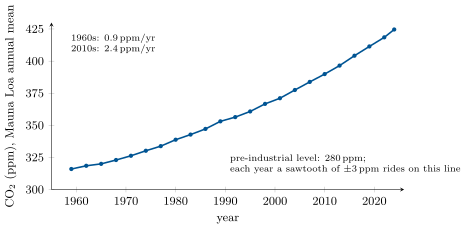
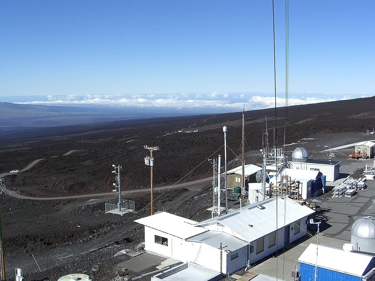
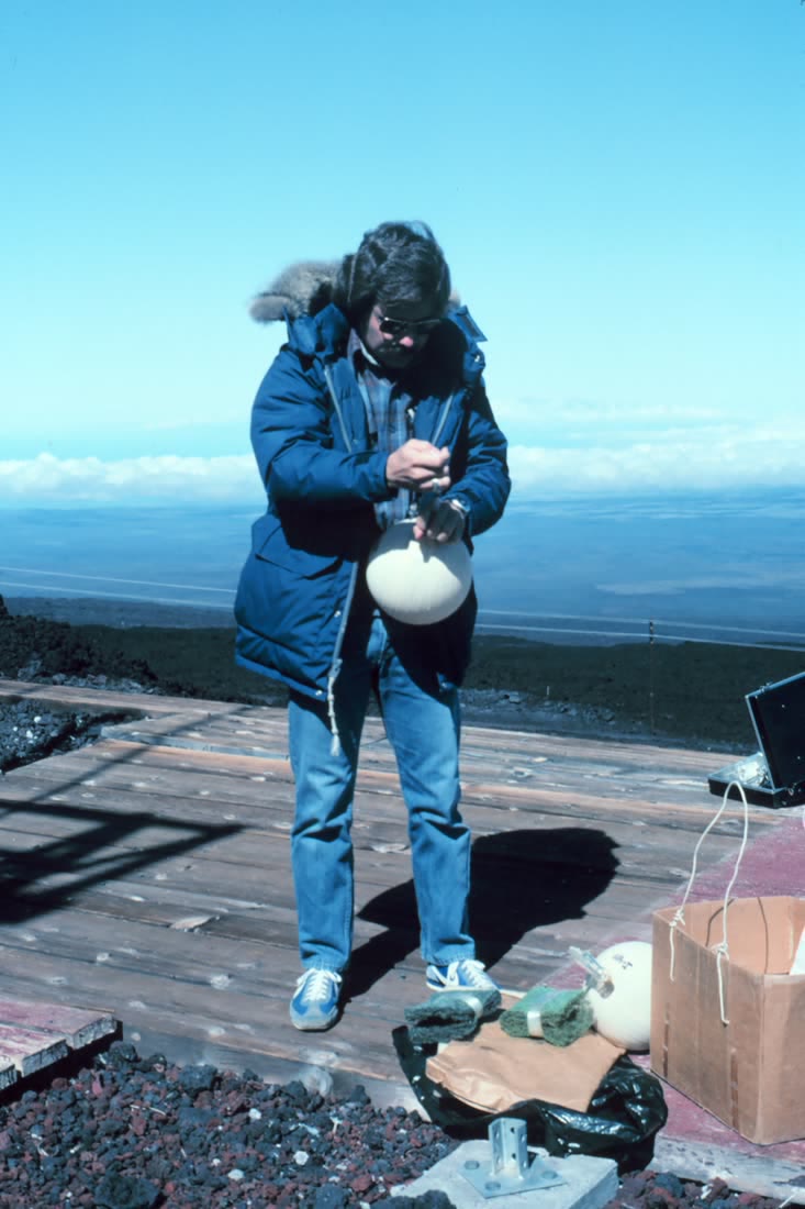
In March 1958 a young chemist named Charles Keeling switched on an infrared gas analyser on the north slope of Mauna Loa, in Hawaii, three and a half kilometres above the Pacific, where the air is as well mixed as air can be. He had expected to measure a constant; within a year he had a sawtooth — carbon dioxide rising every winter and falling every summer as the forests of the northern hemisphere breathed out and in — and within a few years a slope under the sawtooth that has not stopped since. The Keeling curve is the biosphere’s breathing seen from outside, with a fever chart drawn over it. This chapter is about the cycles the curve records: where the carbon, nitrogen, phosphorus and sulfur of living things are stored, how fast they move between reservoirs, what sets those speeds — most of them the metabolisms of Chapter 2 — and what one species has done to each cycle in two hundred years.

25.1 Reservoirs, fluxes and residence times

Definition 25.1 (Reservoir, flux, residence time)

A biogeochemical cycle is the movement of an element between reservoirs (the atmosphere, the ocean, soils, living biomass, rocks) by fluxes measured in mass per year. A reservoir of mass $M$ with total outflow $F$ has a residence time $\tau = M/F$ , the average time an atom spends in it; at steady state inflow equals outflow and $M$ is constant. The cycles are coupled through the stoichiometry of life — the Redfield ratio of marine plankton, $\mathrm{C:N:P} = 106:16:1$ by atoms — so that the supply of the scarcest element sets the rate at which all the others are taken up.

Theorem 25.2 (The one-box model)

If a reservoir loses its content at a rate proportional to what it holds, $F_{\text{out}} = M/\tau$ , and receives a constant inflow $F_{\text{in}}$ , then

\frac{\mathrm{d}M}{\mathrm{d}t} = F_{\text{in}} - \frac{M}{\tau}, \qquad M(t) = M^{*} + (M_0 - M^{*})\,e^{-t/\tau}, \qquad M^{*} = F_{\text{in}}\tau :

the reservoir relaxes to a steady state proportional to its input, with the residence time as the time constant. A step increase in input raises the steady state in proportion and the reservoir follows within a few $\tau$ : a pool with a residence time of days (atmospheric ammonia, the nitrate of a lake in spring) tracks its sources; one with a residence time of centuries (deep-ocean carbon, soil organic matter) integrates them, and the perturbation of a slow pool outlives the perturbation that caused it.

Proof. The equation is linear with constant coefficients: the steady state $M^{*}$ makes the right side zero, and the deviation $m = M - M^{*}$ obeys $\dot m = -m/\tau$ , so $m = m_0 e^{-t/\tau}$ . If a reservoir has several outflows, $\tau$ is set by their sum, $1/\tau = \sum_i 1/\tau_i$ : the fastest sink dominates. ∎

25.2 The carbon cycle

Proposition 25.3 (The carbon budget)

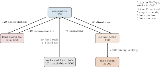
In units of gigatonnes of carbon ( $\mathrm{GtC}$ , $10^{12}$ kg), the main reservoirs are the atmosphere (about 880 in the 2020s, 590 before industry), land plants (450), soils (1700), the surface ocean (900), the deep ocean ( $37\,000$ ) and sedimentary rocks ( $10^{8}$ ); fossil fuels are the fraction of the last that industry can reach, some $5000$ . The natural fluxes are large and nearly balanced: photosynthesis on land takes about 120 a year and respiration and decomposition return it; the ocean surface exchanges about 80 each way with the air. The human flux is small against these — some 10 a year from fossil fuels and 1 from deforestation — but one-way, and the atmosphere has kept about $45\,\%$ of it (the airborne fraction), the ocean taking a quarter and the land, fertilised by the extra $\mathrm{CO_2}$ , the rest. One part per million of atmospheric $\mathrm{CO_2}$ is $2.13\,\mathrm{GtC}$ ; the concentration rose from 280 to $315$ ppm between 1750 and 1958, and from 315 to over $420$ between 1958 and the 2020s, currently by $2.5\,\mathrm{ppm}$ a year. The residence time of a $\mathrm{CO_2}$ molecule in the air, $880/200 \approx 4$ years, is short; the lifetime of the excess, set by the slow mixing into the deep ocean and the slower weathering of rock, is centuries to millennia — a fifth of what is emitted today will still be in the air in ten thousand years.

Evidence. Three signatures show that the added carbon is fossil. Its isotopes: fossil carbon has no $\mathrm{{}^{14}C}$ (it decayed away millions of years ago) and is depleted in $\mathrm{{}^{13}C}$ as all plant carbon is, and the atmosphere has been losing both — the Suess effect, measured in tree rings since the 1950s. Its oxygen: the atmosphere’s $\mathrm{O_2}$ falls in step, by the stoichiometry of combustion, as Keeling’s son showed in the 1990s, which a volcanic or oceanic source would not produce. Its bookkeeping: the sum of coal, oil and gas sold, converted to carbon, exceeds the increase in the air by a factor of two, and the missing half is found in the ocean’s rising dissolved inorganic carbon and falling pH, and in the land sink. The seasonal sawtooth, larger at Barrow in Alaska than at Mauna Loa and nearly absent at the South Pole, is the northern forests’ summer uptake and winter release — a direct measurement of the biosphere’s breathing. ∎

The Keeling curve: annual mean carbon dioxide in the air at Mauna Loa since 1959. The slope has nearly tripled; the seasonal sawtooth on top of it, not shown at this scale, is the northern hemisphere’s summer photosynthesis.

The carbon cycle in round numbers. The natural exchanges are ten times the human flux, but they nearly cancel; the human flux does not.

Where the curve is drawn. Left: the observatory on the north flank of Mauna Loa, 3400\, m up, above the trade-wind inversion that keeps the island’s own air below. Right: a flask sample being taken in 1982; flasks like these, analysed in California, check the continuous analyser and are filled at stations from Alaska to the South Pole. — Where the curve is drawn. Left: the observatory on the north flank of Mauna Loa, $3400\,\mathrm{m}$ up, above the trade-wind inversion that keeps the island’s own air below. Right: a flask sample being taken in 1982; flasks like these, analysed in California, check the continuous analyser and are filled at stations from Alaska to the South Pole.

25.3 The nitrogen cycle

Proposition 25.4 (The nitrogen cycle)

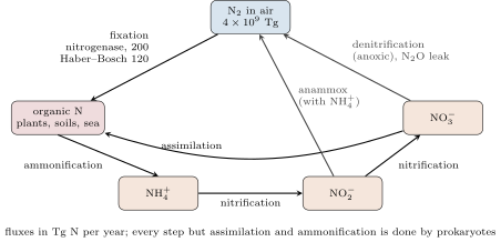
Nitrogen is abundant — the air holds $4\times 10^{9}$ Tg of $\mathrm{N_2}$ — and scarce, because the triple bond of $\mathrm{N_2}$ is opened by only two processes: lightning (a few Tg a year) and biological nitrogen fixation by prokaryotes with nitrogenase, some 100 Tg a year on land and 100 in the sea, at a cost of 16 ATP per $\mathrm{N_2}$ . Fixed nitrogen then runs a redox ladder driven by microbes (Chapter 2): ammonification of dead matter to $\mathrm{NH_4^{+}}$ ; nitrification of $\mathrm{NH_4^{+}}$ to $\mathrm{NO_2^{-}}$ and $\mathrm{NO_3^{-}}$ by aerobic chemolithotrophs; uptake of $\mathrm{NH_4^{+}}$ or $\mathrm{NO_3^{-}}$ by plants and their reduction back to amine; and, where oxygen is absent, denitrification of $\mathrm{NO_3^{-}}$ to $\mathrm{N_2}$ (with $\mathrm{N_2O}$ as a leak) and anammox, the anaerobic oxidation of ammonium by nitrite to $\mathrm{N_2}$ , which together return about as much to the air as fixation takes. The residence time of a nitrogen atom in the biosphere is a few hundred years; in the atmosphere, $4\times 10^{9}/400 \approx 10^{7}$ years. Since 1913 the Haber–Bosch process has fixed nitrogen industrially, now about 120 Tg a year, and cultivated legumes and fossil-fuel combustion add 60 and 30: human activity fixes as much nitrogen as all natural processes together, and feeds half the people alive.

The nitrogen cycle as a redox ladder (plants assimilate ammonium as well as nitrate). Fixation and denitrification, the two doors to the atmosphere, are both microbial; the industrial door now equals the natural one.

Evidence. Hubbard Brook Experimental Forest, New Hampshire: in 1965 one entire watershed was clear-felled and kept bare with herbicide, while a neighbouring one was left intact, and the streams draining each were gauged and analysed for years. The stripped watershed lost nitrate at sixty times the control’s rate — the whole nitrogen capital of the soil, no longer taken up by plants, was nitrified and washed out, taking calcium and potassium with it and acidifying the stream. The experiment showed the cycle’s tightness in an intact forest (a few kilograms of nitrogen lost per hectare per year, against hundreds cycled) and what breaks it. ∎

25.4 Phosphorus and sulfur

Proposition 25.5 (Two cycles without a fast gas)

Phosphorus has no gaseous form. It enters ecosystems by the weathering of apatite in rock, some 20 Tg a year over the whole land surface, is recycled within soils and lakes many times over — a phosphate ion in a lake’s surface water is taken up within hours — and leaves to the sediments, where it stays for the $10^{8}$ years of a rock cycle. Life is therefore phosphorus-thrifty and phosphorus-limited: the residence time in the ocean is some $20\,000$ years, and the deep sea’s phosphate, brought up by upwelling, sets its productivity. Mining now moves about as much phosphorus onto farmland as weathering releases, and its runoff into lakes causes eutrophication: an algal bloom, its decay, the consumption of oxygen, and the death of the fish — Schindler’s whole-lake experiments in Ontario in the 1970s, with one half of a lake fertilised with phosphorus and the other not, showed phosphorus alone to be the trigger, and led to its removal from detergents. Sulfur has both a rock cycle (gypsum, pyrite) and a gas phase: the $\mathrm{SO_2}$ of volcanoes and coal, the $\mathrm{H_2S}$ of anoxic sediments, and dimethyl sulfide from marine plankton, whose oxidation products seed the clouds over the ocean. Coal burning tripled the flux of sulfur to the air in the twentieth century and gave Europe and North America their acid rain; scrubbers reversed it within decades, the cycle’s residence time in the air being a few days.

Two doors of the nitrogen cycle. Left: root nodules of a legume, each a chamber in which rhizobia fix nitrogen for their host. Right: a flooded rice paddy, anoxic below the surface, where denitrification returns nitrogen to the air and methanogens make methane.

25.5 The perturbed planet

Example 25.6 (What the numbers say)

Emissions of $10\,\mathrm{GtC}$ a year with an airborne fraction of $0.45$ leave $4.5\,\mathrm{GtC}$ , or $2.1\,\mathrm{ppm}$ , in the air each year — the observed slope. Cumulative emissions since 1850 are about $700\,\mathrm{GtC}$ , of which $290\,\mathrm{GtC}$ is in the air (140 ppm), the rest in ocean and land. To hold the atmosphere at any level, net emissions must fall to what the slow sinks — deep-ocean mixing and weathering, together under $1\,\mathrm{GtC}$ a year — can take: net zero is not a slogan but the box model’s steady-state condition with a very long $\tau$ . For nitrogen, the doubling of the fixed-nitrogen flux has doubled the nitrate in rivers, produced dead zones at the mouths of the Mississippi and the Baltic, and raised the atmosphere’s $\mathrm{N_2O}$ , a greenhouse gas with a residence time of a century, by a fifth. Chapter 27 follows the consequences for living things.

25.6 Exercises

Exercise 25.1 ★

Define reservoir, flux and residence time, and compute the residence time of carbon in land plants (450 GtC, photosynthesis 120 GtC a year) and in the deep ocean ( $37\,000$ GtC, exchange about 100 GtC a year).

Solution

Solution of Exercise 25.1.

A reservoir is a store of the element (a mass); a flux is a rate of transfer between reservoirs (mass per year); the residence time is the reservoir’s mass divided by its total outflow, the mean time an atom spends there. Land plants: $450/120 \approx 4$ years (a leaf’s carbon, roughly; wood stays for decades and the average hides the spread). Deep ocean: $37000/100 \approx 400$ years — the time before a molecule that has sunk sees the surface again.

Exercise 25.2 ★

Convert $2.5\,\mathrm{ppm}$ a year into GtC, and $10\,\mathrm{GtC}$ of emissions into ppm.

Solution

Solution of Exercise 25.2.

$2.5\times 2.13 = 5.3\,\mathrm{GtC}$ a year. $10/2.13 = 4.7\,\mathrm{ppm}$ — if all of it stayed in the air; at the $45\,\%$ airborne fraction, $2.1\,\mathrm{ppm}$ .

Exercise 25.3 ★

Name the two natural processes that open $\mathrm{N_2}$ , the process that returns it, and the three redox steps in between, with the organisms responsible.

Solution

Solution of Exercise 25.3.

Opening: biological fixation by nitrogenase (cyanobacteria, rhizobia, Azotobacter, Frankia) and lightning. Return: denitrification (facultative anaerobes such as Pseudomonas and Paracoccus in anoxic soil and sediment) and anammox (planctomycetes). Between: ammonification of organic nitrogen to ammonium by decomposers (fungi, bacteria); nitrification of ammonium to nitrite (Nitrosomonas, ammonia-oxidising archaea) and of nitrite to nitrate (Nitrobacter); and assimilation of ammonium or nitrate by plants and microbes.

Exercise 25.4 ★

Why does phosphorus limit productivity more often than nitrogen over geological time, and nitrogen more often than phosphorus in a given season?

Solution

Solution of Exercise 25.4.

Over geological time, nitrogen can always be made from the inexhaustible $\mathrm{N_2}$ of the air by fixers, which are favoured whenever nitrogen is short; phosphorus has no such reservoir and its supply is fixed by weathering, so the long-run ceiling on productivity is phosphorus. Within a season, fixation is slow and costly, and most plants cannot do it, so the nitrogen at hand is what limits growth here and now — which is why fertiliser is mostly nitrogen.

Exercise 25.5 ★★

A lake of $10^{7}\,\mathrm{m}^{3}$ receives $2\,\mathrm{t}$ of phosphorus a year and flushes $20\,\%$ of its water annually. Compute its steady state phosphorus concentration and the time to reach $90\,\%$ of it after the input starts. What if the input is halved?

Solution

Solution of Exercise 25.5.

$\tau = 1/0.2 = 5$ years; $M^{*} = F\tau = 10\,\mathrm{t}$ , that is $1\,\mathrm{g}/\mathrm{m}^{3} = 1000\,\mathrm{mg}/\mathrm{m}^{3}$ , grossly eutrophic. Time to $90\,\%$ : $\tau\ln 10 = 11.5$ years. Halving the input halves the steady state, to $500\,\mathrm{mg}/\mathrm{m}^{3}$ , reached on the same time scale.

Exercise 25.6 ★★

From the Keeling data, compute the mean growth rate of $\mathrm{CO_2}$ in the 1960s (316 to $325\,\mathrm{ppm}$ over ten years) and in the 2010s (390 to 411 over nine years), in ppm a year and in GtC a year.

Solution

Solution of Exercise 25.6.

1960s: $0.9\,\mathrm{ppm}/\mathrm{yr}$ , $1.9\,\mathrm{GtC}/\mathrm{yr}$ . 2010s: $2.3\,\mathrm{ppm}/\mathrm{yr}$ , $5.0\,\mathrm{GtC}/\mathrm{yr}$ . The growth rate has increased two and a half times, in step with emissions.

Exercise 25.7 ★★

The seasonal sawtooth at Mauna Loa has an amplitude of about $6\,\mathrm{ppm}$ peak to trough. Convert to GtC and compare with the annual net primary production of the northern hemisphere’s land, about $35\,\mathrm{GtC}$ . Why is the sawtooth so much smaller?

Solution

Solution of Exercise 25.7.

$6\,\mathrm{ppm}$ is $13\,\mathrm{GtC}$ , against a net primary production of $35\,\mathrm{GtC}$ : the sawtooth is a third of it. It is smaller because respiration and decomposition continue through the summer (the sawtooth records the net uptake, not the gross), because the southern hemisphere’s seasons are opposite and partly cancel, and because the ocean damps the swing.

Exercise 25.8 ★★

Nitrogenase spends 16 ATP per $\mathrm{N_2}$ . For a legume fixing $200\,\mathrm{kg}$ of nitrogen per hectare per year, compute the moles of $\mathrm{N_2}$ fixed and the ATP spent, and the mass of glucose that ATP represents (about 30 ATP per glucose). What fraction of a $10\,\mathrm{t}/\mathrm{ha}$ crop’s photosynthate is that?

Solution

Solution of Exercise 25.8.

$200\,\mathrm{kg}/(28\,\mathrm{g}/\mathrm{mol}) = 7100$ mol of $\mathrm{N_2}$ ; $16\times 7100 = 114\,000$ mol ATP; $/30 = 3800$ mol glucose, $690\,\mathrm{kg}$ . A crop that builds $10\,\mathrm{t}$ of dry matter fixes roughly $15\text{ to }20\,\mathrm{t}$ of sugar once respiration is counted, so fixation costs it some $4\,\%$ of its photosynthate — the price of independence from the soil’s nitrogen.

Exercise 25.9 ★★

Plankton grow at the Redfield ratio $\mathrm{C:N:P} = 106:16:1$ . Seawater at depth holds $2.2\,\text{µ}\mathrm{mol}/\mathrm{kg}$ phosphate and $32\,\text{µ}\mathrm{mol}/\mathrm{kg}$ nitrate. Which runs out first when a parcel is brought to the surface, and how much carbon is fixed before it does?

Solution

Solution of Exercise 25.9.

Ratio available $\mathrm{N:P} = 32/2.2 = 14.5$ , below the Redfield 16: nitrate runs out first, with $0.2\,\text{µ}\mathrm{mol}/\mathrm{kg}$ of phosphate left over. Carbon fixed: $32\times 106/16 = 212\,\text{µ}\mathrm{mol}/\mathrm{kg}$ , about $2.5\,\mathrm{mg}$ of carbon per kilogram of water.

Exercise 25.10 ★★★

Treat the atmosphere as a box with excess carbon $E$ removed at rate $E/\tau$ by the sinks and fed by emissions $Q$ . With $\tau = 50$ years and $Q = 10\,\mathrm{GtC}/\mathrm{yr}$ , what is the steady-state excess and what ppm does it correspond to? Explain why the real answer is worse.

Solution

Solution of Exercise 25.10.

$E^{*} = Q\tau = 500\,\mathrm{GtC}$ , $235\,\mathrm{ppm}$ above the pre-industrial 285: about $520\,\mathrm{ppm}$ . Worse in reality because the sinks are not a single fast pool: the surface ocean saturates (its capacity to take up $\mathrm{CO_2}$ falls as its carbonate is used), the land sink weakens with warming, and the true removal has a slow component — deep-ocean mixing and rock weathering — with time constants of a thousand to a hundred thousand years, so a fraction of the excess does not relax on any $\tau$ of decades.

Exercise 25.11 ★★★

Bomb tests doubled the atmosphere’s $\mathrm{{}^{14}C}$ in 1963; the excess then fell by half every 11 years or so, although $\mathrm{{}^{14}C}$ has a half-life of 5730 years. Explain what was measured, and what the 11 years tells you about the carbon cycle.

Solution

Solution of Exercise 25.11.

What was measured is the exchange of atmospheric $\mathrm{CO_2}$ with the ocean and biosphere, not decay: the bomb $\mathrm{{}^{14}C}$ was diluted into the much larger pools of the surface ocean and the plants and soils, which then returned ordinary carbon. The 11-year half-life of the excess (an e-folding time of about 16 years) is the time scale of that exchange — the turnover of the atmosphere’s carbon with respect to the surface ocean and land, longer than the four-year gross residence time because much of what leaves comes straight back.

Exercise 25.12 ★★★

“Humans have doubled the nitrogen cycle and merely nudged the carbon cycle.” Discuss with numbers: fluxes fixed, fractions of the natural flux, and the reservoirs affected.

Solution

Solution of Exercise 25.12.

Nitrogen: natural fixation about 200 Tg a year; human fixation (Haber–Bosch 120, crops 60, combustion 30) about 210: the flux is doubled, and the reservoirs affected — soils, rivers, coastal seas, the $\mathrm{N_2O}$ of the air — are small and fast, so the change shows within decades, while the $\mathrm{N_2}$ reservoir is untouched. Carbon: human emissions of 11 GtC a year are only $5\,\%$ of the gross natural exchange of about 200, so the flux is nudged; but the natural fluxes cancel and the human one does not, and it has raised the atmospheric reservoir by $50\,\%$ — the small nudge has a large cumulative effect on a reservoir with a slow ultimate sink. Which cycle is “more perturbed” depends on whether one counts fluxes or accumulation.

25.7 Problem: The Carbon Budget of a Century

Problem 25.1

Weekend problem — a century of emissions passed through the box model of the atmosphere, the ocean’s share and the land’s, the nitrogen cascade from a fertilised field to a dead zone, and a lake’s phosphorus budget, ending on the airborne fraction, the atmospheric concentration in 2100, and the nitrogen lost per hectare

Data. Atmosphere in 1850: $285\,\mathrm{ppm}$ ; $1\,\mathrm{ppm}$ $= 2.13\,\mathrm{GtC}$ . Cumulative emissions 1850–2020: $700\,\mathrm{GtC}$ ; atmospheric $\mathrm{CO_2}$ in 2020: $412\,\mathrm{ppm}$ . A field of $1\,\mathrm{ha}$ receives $150\,\mathrm{kg}$ of nitrogen fertiliser a year; the crop takes up $60\,\%$ , $25\,\%$ is denitrified, the rest leaches. A lake of $5 \times 10^{7}\,\mathrm{m}^{3}$ flushes a tenth of its water a year and receives $5\,\mathrm{t}$ of phosphorus a year.

Part I — The airborne fraction.

Compute the atmospheric carbon in 1850 and in 2020, and the increase in GtC.
Compute the airborne fraction over 1850–2020.
Where is the rest? Give the two sinks and, from the proposition, their approximate shares.
If the ocean has taken $25\,\%$ of the emissions, by how much has its dissolved inorganic carbon, $38\,000\,\mathrm{GtC}$ , risen in relative terms? Why does the surface ocean nonetheless acidify measurably?
Why does the airborne fraction stay roughly constant while emissions grow exponentially? (Consider the box model with $Q \propto e^{t/T}$ and a sink $E/\tau$ .)
What would the airborne fraction become if emissions were held constant for many centuries?

Part II — The century ahead. Model the excess carbon $E$ (above the 1850 level) with $\mathrm{d}E/\mathrm{d}t = Q - E/\tau$ , $\tau = 100$ years.

Compute the excess in 2020 in GtC.
With $Q$ held at $10\,\mathrm{GtC}/\mathrm{yr}$ , compute the steady-state excess and the concentration it implies.
Solve for $E(t)$ from 2020 with $Q = 10$ and give $E$ in 2100 and the concentration.
Now let $Q$ fall linearly to zero between 2020 and 2070 and stay at zero. Compute $E$ in 2070 (integrate the equation; the particular solution for a linear $Q$ is linear plus a constant) and in 2100.
Compare the two concentrations in 2100.
Why is a single $\tau$ optimistic for the second scenario?

Part III — The nitrogen cascade.

Compute the nitrogen taken up by the crop, denitrified and leached, per hectare per year.
The leached nitrogen reaches a river as nitrate and then the sea, where plankton use it at the Redfield ratio. How much carbon does it allow the plankton to fix?
That carbon sinks and is respired at depth, consuming oxygen at 1 $\mathrm{O_2}$ per C. Compute the oxygen consumed, in moles and in kilograms.
A cubic metre of seawater holds about $0.25\,\mathrm{mol}$ of $\mathrm{O_2}$ when saturated. How many cubic metres of bottom water does one hectare’s leaching deoxygenate?
The denitrified fraction escapes partly as $\mathrm{N_2O}$ , $1\,\%$ of the nitrogen denitrified. Compute the $\mathrm{N_2O}$ per hectare per year, and its warming equivalent in $\mathrm{CO_2}$ ( $\mathrm{N_2O}$ is 270 times $\mathrm{CO_2}$ per kilogram).
Compare with the $\mathrm{CO_2}$ emitted to make the fertiliser (about $4\,\mathrm{kg}$ of $\mathrm{CO_2}$ per kilogram of nitrogen by Haber–Bosch).

Part IV — The lake.

Compute the lake’s phosphorus residence time if the only loss is flushing, and its steady-state concentration in $\mathrm{mg}/\mathrm{m}^{3}$ .
Lakes with more than $30\,\mathrm{mg}/\mathrm{m}^{3}$ of phosphorus are eutrophic. Is this one?
Sedimentation removes phosphorus with its own time constant of 5 years. Recompute the residence time and the concentration.
The input is cut to $1\,\mathrm{t}$ a year. Compute the new steady state and the time to get within $10\,\%$ of it.
Why do many lakes recover more slowly than this calculation predicts?
Compute the carbon the lake’s phosphorus can build into plankton each year at the Redfield ratio, from the $5\,\mathrm{t}$ input.
State the result: the airborne fraction, the two concentrations in 2100, and the nitrogen leached per hectare.

Solution

Solution of Problem 25.1.

1. $285\times 2.13 = 607\,\mathrm{GtC}$ ; $412\times 2.13 = 878\,\mathrm{GtC}$ ; increase $271\,\mathrm{GtC}$ . 2. $271/700 = 0.39$ (the fraction over recent decades, with land-use emissions counted, is nearer $0.45$ ). 3. The ocean, about a quarter of emissions, and the land (forest regrowth and $\mathrm{CO_2}$ fertilisation), about a third; the remainder of the $430\,\mathrm{GtC}$ not in the air. 4. $175/38000 = 0.5\,\%$ — negligible for the whole ocean; but the uptake has so far entered mainly the surface layer ( $900\,\mathrm{GtC}$ ), where it is a rise of a tenth or more, and the carbonate chemistry turns a small rise in dissolved $\mathrm{CO_2}$ into a larger rise in hydrogen-ion concentration: surface pH has fallen by $0.1$ , a $30\,\%$ rise in acidity. 5. With $Q = Q_0 e^{t/T}$ , try $E = Ae^{t/T}$ : $A/T = Q_0 - A/\tau$ , so $A = Q_0\tau T/(\tau + T)$ and the airborne fraction $\dot E/Q = \tau/(\tau + T)$ is constant. Emissions growing at $2\,\%$ a year ( $T = 50$ ) with $\tau = 40$ give $0.44$ : the fraction is constant because sink and source grow together. 6. With $Q$ constant, $E \to Q\tau$ and $\dot E \to 0$ : the airborne fraction falls toward zero as the sinks catch up — in the one-box model; in reality the sinks saturate and the fraction falls more slowly. 7. $271\,\mathrm{GtC}$ . 8. $E^{*} = 10\times 100 = 1000\,\mathrm{GtC}$ : $285 + 1000/2.13 = 755\,\mathrm{ppm}$ . 9. $E(t) = 1000 + (271 - 1000)e^{-t/100}$ ; at $t = 80$ , $E = 1000 - 729\times 0.449 = 672\,\mathrm{GtC}$ : $600\,\mathrm{ppm}$ . 10. $Q = 10(1 - t/50)$ : particular solution $E_p = at + b$ with $a = -20$ , $b = 3000$ (from $a = 10 - b/\tau$ and $0 = -0.2 - a/\tau$ ); $E = 3000 - 20t + (271 - 3000)e^{-t/100}$ . At $t = 50$ : $2000 - 2729\times 0.607 = 344\,\mathrm{GtC}$ , $447\,\mathrm{ppm}$ . Then $E$ decays freely: at $t = 80$ , $344\,e^{-0.3} = 255\,\mathrm{GtC}$ , $405\,\mathrm{ppm}$ . 11. $600\,\mathrm{ppm}$ against $405\,\mathrm{ppm}$ : the second scenario returns the air, by 2100, nearly to where it is today. 12. The single $\tau$ makes the sinks keep working at the same rate on a shrinking excess; in reality the fast sinks (the mixed layer, the growing forests) have already taken what they can and the remaining removal is by slow deep-ocean mixing and weathering with $\tau$ of centuries to millennia, so the decline after net zero is far slower — the concentration stays roughly constant for centuries rather than falling. 13. Crop $90\,\mathrm{kg}$ ; denitrified $37.5\,\mathrm{kg}$ ; leached $22.5\,\mathrm{kg}$ of nitrogen per hectare per year. 14. $22.5\,\mathrm{kg}/14\,\mathrm{g}/\mathrm{mol} = 1600$ mol N; carbon $1600\times 106/16 = 10\,600$ mol, $128\,\mathrm{kg}$ . 15. $10\,600$ mol $\mathrm{O_2}$ , $340\,\mathrm{kg}$ . 16. $10\,600/0.25 = 42\,000$ $\mathrm{m}^{3}$ : one hectare’s leaching can strip the oxygen from forty thousand cubic metres of bottom water each year — and the Mississippi drains a hundred million hectares. 17. $37.5\times 0.01 = 0.375\,\mathrm{kg}$ of nitrogen as $\mathrm{N_2O}$ , that is $0.375\times 44/28 = 0.59\,\mathrm{kg}$ of $\mathrm{N_2O}$ ; $\times 270 = 160\,\mathrm{kg}$ of $\mathrm{CO_2}$ equivalent. 18. $150\times 4 = 600\,\mathrm{kg}$ of $\mathrm{CO_2}$ : the manufacture outweighs the field’s $\mathrm{N_2O}$ by four to one, and the two together are three quarters of a tonne per hectare per year. 19. $\tau = 10$ years; $M^{*} = 5\times 10 = 50\,\mathrm{t}$ ; concentration $50/(5\times 10^{7}) = 1\,\mathrm{g}/\mathrm{m}^{3} = 1000\,\mathrm{mg}/\mathrm{m}^{3}$ . 20. Thirty times over the threshold: severely eutrophic. 21. $1/\tau = 0.1 + 0.2 = 0.3$ : $\tau = 3.3$ years; $M^{*} = 5/0.3 = 16.7\,\mathrm{t}$ , $330\,\mathrm{mg}/\mathrm{m}^{3}$ . 22. $M^{*} = 1/0.3 = 3.3\,\mathrm{t}$ , $67\,\mathrm{mg}/\mathrm{m}^{3}$ — still eutrophic; within $10\,\%$ after $\tau\ln 10 = 7.7$ years. 23. The sediment is not a one-way sink: phosphorus stored in it over the eutrophic years is released back under the anoxic conditions that eutrophication itself creates (iron-bound phosphate dissolves when the iron is reduced), so the lake feeds itself for years after the external input is cut — internal loading, a second reservoir with a long residence time. 24. $5000\,\mathrm{kg}/31\,\mathrm{g}/\mathrm{mol} = 1.6\times 10^{5}$ mol P; carbon $\times 106 = 1.7\times 10^{7}$ mol, $205\,\mathrm{t}$ of carbon a year — $20\,\mathrm{g}/\mathrm{m}^{2}$ over the lake’s surface if it is $5\,\mathrm{m}$ deep, a heavy bloom. 25. Airborne fraction $0.39$ over 1850–2020; in 2100, $600\,\mathrm{ppm}$ with emissions held at $10\,\mathrm{GtC}/\mathrm{yr}$ and $405\,\mathrm{ppm}$ with emissions cut to zero by 2070 (an optimistic single- $\tau$ model); nitrogen leached $22.5\,\mathrm{kg}$ per hectare per year.

Terms defined in this chapter

Reservoir, flux, residence time

See all 479 terms in the glossary