University Physics — Year 3 · Bachelor Year 3

10Quantum Angular Momentum

Point a radio telescope at a dark patch of sky and tune it to $115\,\mathrm{GHz}$ : a bright, needle-sharp line appears — carbon monoxide molecules, ten kelvin above absolute zero, stepping down one rung of a ladder of rotational states. Their tumbling, like everything that turns in quantum mechanics, is quantised twice over: the magnitude of the angular momentum can only be $\sqrt{l(l+1)}\,\hbar$ , and its component along any chosen axis only $m\hbar$ . This chapter derives that double quantisation — once algebraically, from the commutators inherited from the Poisson brackets of Chapter 2, and once concretely, as the spherical harmonics that shape every atomic orbital. The algebra will hand us more than we ask: it permits half-integer values that no orbital motion can realise, a vacancy nature fills two chapters from now with spin. On the way we meet the molecules’ rotational ladders — the millimetre-wave lines by which astronomers weigh the galaxies’ cold gas — and the magnetic moments by which angular momentum first showed itself split.

10.1 The algebra of rotation

Definition 10.1 (Angular momentum operators)

Orbital angular momentum is the operator $\hat{\vect L} = \hat{\vect r}\wedge\hat{\vect p}$ , componentwise $\hat L_z = \hat x\hat p_y - \hat y\hat p_x$ and cyclic. From $[\hat x, \hat p_x] = \iu\hbar$ :

[\hat L_x, \hat L_y] = \iu\hbar\,\hat L_z \quad\text{(and cyclic)} , \qquad [\hat L^2, \hat L_z] = 0 :

the components are mutually incompatible — no state has two of them sharp — but the total square is compatible with any one of them: the pair $(\hat L^2, \hat L_z)$ is the standard choice of labels. These commutators are exactly $\iu\hbar$ times the Poisson brackets computed in Example 2.12: Dirac’s dictionary at work.

Theorem 10.2 (The spectrum, from the algebra alone)

Let $\hat J_x, \hat J_y, \hat J_z$ be any three Hermitian operators obeying the commutation relations above. Then the joint eigenvalues of $(\hat J^2, \hat J_z)$ are

\hat J^2:\ j(j+1)\hbar^2 , \qquad \hat J_z:\ m\hbar , \quad m = -j, -j+1, \dots, +j ,

where $j$ is a non-negative integer or half-integer: $2j + 1$ values of $m$ for each $j$ . The ladder operators $\hat J_\pm = \hat J_x \pm \iu\hat J_y$ step $m$ by $\pm1$ at fixed $j$ :

\hat J_\pm\ket{j,m} = \hbar\sqrt{j(j+1) - m(m\pm1)}\,\ket{j,m\pm1} .

Partial proof. $[\hat J_z, \hat J_\pm] = \pm\hbar\hat J_\pm$ : acting with $\hat J_\pm$ shifts the $\hat J_z$ eigenvalue by $\pm\hbar$ , at fixed $\hat J^2$ (which commutes with everything built from the $\hat J_i$ ). The norm $\|\hat J_\pm\ket{j,m}\|^2 = \hbar^2[j(j+1) - m(m\pm1)]$ (computed from $\hat J_\mp\hat J_\pm = \hat J^2 - \hat J_z^2 \mp \hbar\hat J_z$ ) must stay non-negative: the ladder must terminate above at some $m_{\max}$ with $m_{\max}(m_{\max}+1) = j(j+1)$ , i.e. $m_{\max} = j$ , and below at $m_{\min} = -j$ . Climbing from $-j$ to $+j$ in unit steps forces $2j$ to be a non-negative integer. The eigenvalue notation $j(j+1)\hbar^2$ is thereby justified after the fact. ∎

Remark 10.3 (A vacancy in the catalogue)

The algebra allows $j = \tfrac12, \tfrac32, \dots$ — ladders with an even number of rungs. Orbital motion, we show next, uses only integers. Nature, however, wastes nothing: the electron itself carries $j = \tfrac12$ , with no orbit behind it (Chapter 12); the algebra derived here, unchanged, will run atomic magnetism, nuclear spins and the qubit.

10.2 Orbital angular momentum: spherical harmonics

Proposition 10.4 (Spherical harmonics)

In spherical coordinates $\hat L_z = -\iu\hbar\,\partial_\varphi$ , and the joint eigenfunctions of $(\hat L^2, \hat L_z)$ on the sphere are the spherical harmonics $Y_l^m(\theta, \varphi)$ :

\hat L^2\,Y_l^m = l(l+1)\hbar^2\,Y_l^m , \qquad \hat L_z\,Y_l^m = m\hbar\,Y_l^m ,

with $l = 0, 1, 2, \dots$ integer — single-valuedness of $\eu^{\iu m\varphi}$ forces integer $m$ , hence integer $l$ . The first few, up to normalisation: $Y_0^0 = \text{const}$ (the $s$ shape, a sphere); $Y_1^0 \propto \cos\theta$ and $Y_1^{\pm1} \propto \sin\theta\,\eu^{\pm\iu\varphi}$ (the $p$ shapes, two lobes); $Y_2^0 \propto 3\cos^2\theta - 1$ and its partners (the $d$ family). Parity: $Y_l^m(-\vect r$ direction $) = (-1)^l\,Y_l^m$ .

Proof. Admitted at this level. ∎

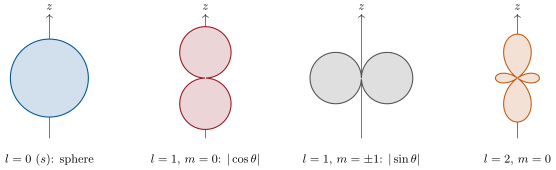
Polar diagrams of |Y_lm( )| (section in a plane containing the z axis; the full shape is the figure of revolution). These angular skeletons, independent of any potential, will dress every atom in . — Polar diagrams of $|Y_l^m(\theta)|$ (section in a plane containing the $z$ axis; the full shape is the figure of revolution). These angular skeletons, independent of any potential, will dress every atom in Chapter 11.

Example 10.5 (The rigid rotor and its ladder)

A diatomic molecule tumbling with moment of inertia $I$ has $\hat H = \hat L^2/2I$ : energies

E_J = \frac{\hbar^2}{2I}\,J(J+1) = B\,J(J+1) , \qquad J = 0, 1, 2, \dots

each $(2J+1)$ -fold degenerate. Photon absorption obeys $\Delta J = \pm1$ , so the absorption frequencies are $\nu_{J+1\leftarrow J} = 2B(J+1)/h$ : a comb of equally spaced lines — the signature by which a rotational spectrum is recognised at a glance. For carbon monoxide, $B/h = 57.6\,\mathrm{GHz}$ : the fundamental line falls at $115\,\mathrm{GHz}$ ( $\lambda = 2.6\,\mathrm{mm}$ ), the workhorse line of millimetre radio astronomy (Problem 10.1).

10.3 Central potentials, completed

Theorem 10.6 (Separation in any central potential)

For $V(r)$ , the stationary states can be taken as

\psi(\vect r) = \frac{u(r)}{r}\,Y_l^m(\theta, \varphi) ,

where $u$ solves the one-dimensional radial equation

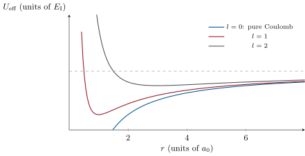
-\frac{\hbar^2}{2m}\,u'' + \Big[V(r) + \frac{\hbar^2\,l(l+1)}{2mr^2}\Big]u = E\,u , \qquad u(0) = 0 .

The angular problem is solved once and for all by the $Y_l^m$ ; each $l$ adds the repulsive centrifugal barrier $\hbar^2l(l+1)/2mr^2$ — the quantum version of the effective potential of Example 1.12 — and every level of given $l$ is $(2l+1)$ -fold degenerate, because no central force can care about the orientation of the $z$ axis. The $s$ -wave trick of Proposition 7.8 was the $l = 0$ row of this theorem.

Partial proof. The Laplacian splits as $\Delta = \tfrac1r\partial_r^2(r\,\cdot) - \hat L^2/\hbar^2r^2$ (admitted; it is the statement that $\hat L^2$ is the angular part of $-\hbar^2\Delta$ ). Insert $\psi = (u/r)Y_l^m$ and use the eigenvalue of $\hat L^2$ : the stated equation. The degeneracy follows because $\hat H$ commutes with all three $\hat L_i$ , whose ladder operators move $m$ without changing the energy. ∎

Effective radial potentials of the Coulomb problem: the centrifugal barrier 2l(l+1)/2mr2 walls off the origin for l 1. Only s states touch the nucleus — with consequences from atomic spectra to radioactive electron capture. — Effective radial potentials of the Coulomb problem: the centrifugal barrier $\hbar^2l(l+1)/2mr^2$ walls off the origin for $l \ge 1$ . Only $s$ states touch the nucleus — with consequences from atomic spectra to radioactive electron capture.

10.4 Magnetic moments: angular momentum made visible

Proposition 10.7 (Orbital magnetic moment and the Zeeman effect)

A particle of charge $q$ and mass $m$ with orbital angular momentum $\hat{\vect L}$ carries the magnetic moment

\hat{\vect\mu} = \frac{q}{2m}\,\hat{\vect L} ;

for the electron, the natural unit is the Bohr magneton $\mu_{\text{B}} = e\hbar/2m_{\text{e}} = 5.79 \times 10^{-5}\,\mathrm{eV}/\mathrm{T}$ (compare Exercise 7.5). In a field $B\vect e_z$ the energy $-\hat{\vect\mu}\cdot\vect B$ shifts each level by $+m\,\mu_{\text{B}}B$ (electron charge negative): a level of given $l$ splits into its $2l + 1$ components — the Zeeman effect, the first direct display of the quantisation of $m$ , and the reason $m$ is called the magnetic quantum number. At $B = 1\,\mathrm{T}$ the splitting is $58\,\text{µ}\mathrm{eV}$ : small beside optical energies, easily resolved as a shift of spectral lines — and, read in reverse, a magnetometer: the Zeeman splitting of sunlight’s lines maps the magnetic fields of sunspots.

Partial proof. Classically a charge on an orbit is a current loop: $\mu = IA = (qv/2\pi r)(\pi r^2) = qL/2m$ ; the operator statement inherits it (and follows from the $\hat{\vect A}$ coupling of Proposition 1.16). The energy shift is first-order perturbation theory, anticipated here and justified in Chapter 13. ∎

“Space quantisation” for l = 2: the angular momentum vector has length √l(l+1)\, = √6\, but can offer the z axis only the five projections m — never its full length: since the components are incompatible, L can never lie exactly along any axis. — “Space quantisation” for $l = 2$ : the angular momentum vector has length $\sqrt{l(l+1)}\,\hbar = \sqrt6\,\hbar$ but can offer the $z$ axis only the five projections $m\hbar$ — never its full length: since the components are incompatible, $\vect L$ can never lie exactly along any axis.

Method 10.8 (Angular momentum in practice)

(1) Label states by $(l, m)$ — or $(j, m)$ for the abstract algebra — and never ask for two components at once. (2) Matrix elements: use the ladder formulas; $\hat L_x = (\hat L_+ + \hat L_-)/2$ . (3) Central potential: quote the $Y_l^m$ , solve only the radial equation with the centrifugal barrier. (4) Rotational energies: $BJ(J+1)$ , lines at $2B(J+1)$ — extract $B$ , hence bond lengths, from equal spacings. (5) Magnetic questions: convert angular momenta to moments at $\mu_{\text{B}}$ per $\hbar$ , energies at $\mu_{\text{B}}B$ per unit $m$ .

10.5 Exercises

Exercise 10.1 ★

(a) Derive $[\hat L_x, \hat L_y] = \iu\hbar\hat L_z$ from the canonical commutators. (b) Show $[\hat L^2, \hat L_z] = 0$ . (c) Show $[\hat L_z, \hat x] = \iu\hbar\hat y$ : what does $\hat L_z$ generate? (d) Why do the three components admit no common eigenbasis — except for one particular state (which)?

Solution

Solution of Exercise 10.1.

(a) $[\hat y\hat p_z - \hat z\hat p_y,\ \hat z\hat p_x - \hat x\hat p_z]$ : only the terms sharing a $\hat z, \hat p_z$ pair survive, giving $\iu\hbar(\hat x\hat p_y - \hat y\hat p_x)$ . (b) $[\hat L^2, \hat L_z] = \sum_i[\hat L_i^2, \hat L_z] = \hat L_x[\hat L_x, \hat L_z] + [\hat L_x, \hat L_z]\hat L_x + (x \to y)$ : the four terms cancel pairwise. (c) $[\hat L_z, \hat x] = \iu\hbar\hat y$ : $\hat L_z$ generates rotations about $z$ — of operators as of states. (d) Common sharpness of two components forces (by the commutator) sharpness of the third with value zero for all three: only $l = 0$ achieves it.

Exercise 10.2 ★

For $l = 1$ , in the basis $\{\ket{1,1}, \ket{1,0}, \ket{1,-1}\}$ : (a) write the matrix of $\hat L_z$ ; (b) use the ladder formula to write $\hat L_+$ and $\hat L_-$ ; (c) assemble $\hat L_x$ and check its eigenvalues are $\hbar, 0, -\hbar$ ; (d) a state with $L_x = +\hbar$ is measured along $z$ : give the probabilities of the three outcomes.

Solution

Solution of Exercise 10.2.

(a) $\hat L_z = \hbar\operatorname{diag}(1, 0, -1)$ . (b) $\hat L_+ = \hbar\sqrt2\,\begin{pmatrix}0&1&0\\0&0&1\\0&0&0 \end{pmatrix}$ , $\hat L_-$ its transpose. (c) $\hat L_x = \dfrac{\hbar}{\sqrt2}\begin{pmatrix}0&1&0\\1&0&1\\0&1&0 \end{pmatrix}$ : characteristic polynomial $\lambda(\lambda^2 - \hbar^2)$ . (d) The $L_x = +\hbar$ eigenvector is $\tfrac12(1, \sqrt2, 1)$ : probabilities $\tfrac14, \tfrac12, \tfrac14$ for $m = +1, 0, -1$ .

Exercise 10.3 ★

Carbon monoxide: bond length $0.113\,\mathrm{nm}$ , reduced mass $1.14 \times 10^{-26}\,\mathrm{kg}$ . (a) Compute $I$ and $B = \hbar^2/2I$ in meV. (b) The frequency and wavelength of the $J = 1 \leftarrow 0$ line. (c) The next two lines. (d) An astronomer measures the comb spacing to five digits: what molecular quantity does she obtain, and to what precision?

Solution

Solution of Exercise 10.3.

(a) $I = \mu r_0^2 = 1.46 \times 10^{-46}\,\mathrm{kg}\,\mathrm{m}^{2}$ ; $B = \hbar^2/2I = 3.8 \times 10^{-23}\,\mathrm{J} = 0.24\,\mathrm{meV}$ . (b) $2B/h = 115\,\mathrm{GHz}$ , $\lambda = 2.6\,\mathrm{mm}$ . (c) $231\,\mathrm{GHz}$ and $346\,\mathrm{GHz}$ . (d) The spacing gives $B$ , hence $I = \mu r_0^2$ : the bond length of a molecule light-years away, to roughly half the spacing’s relative precision.

Exercise 10.4 ★

A particle is in a state of $l = 2$ . (a) List the possible outcomes of measuring $L_z$ . (b) The smallest angle between $\vect L$ and the $z$ axis, using $\cos\theta = m/\sqrt{l(l+1)}$ : evaluate it. (c) Why can the angle never be zero? (d) Show the minimal angle tends to zero as $l \to \infty$ : classical vectors recovered.

Solution

Solution of Exercise 10.4.

(a) $m\hbar$ with $m = -2 \dots 2$ . (b) $\cos\theta = 2/\sqrt6$ : $\theta = 35.3^\circ$ . (c) Perfect alignment would make $L_x = L_y = 0$ sharp together with $L_z$ — forbidden by the commutators except in the trivial $l = 0$ case. (d) $l/\sqrt{l(l+1)} \to 1$ : for large $l$ the cone closes onto the axis and the classical arrow returns.

Exercise 10.5 ★★

The angular part of $-\hbar^2\Delta$ is $\hat L^2$ , with

\hat L^2 = -\hbar^2\Big[\frac{1}{\sin\theta}\,\partial_\theta (\sin\theta\,\partial_\theta) + \frac{1}{\sin^2\theta}\,\partial_\varphi^2\Big] .

(a) Verify that $Y_1^0 \propto \cos\theta$ has $\hat L^2$ -eigenvalue $2\hbar^2$ . (b) Verify $Y_1^{\pm1} \propto \sin\theta\, \eu^{\pm\iu\varphi}$ likewise, and their $\hat L_z$ eigenvalues. (c) Check the parities. (d) Why must $\braket{Y_1^0}{Y_1^1} = 0$ without computing any integral?

Solution

Solution of Exercise 10.5.

(a) With no $\varphi$ dependence, the operator gives $-\hbar^2(\sin\theta)^{-1}\partial_\theta(\sin\theta\,(-\sin\theta)) = 2\hbar^2\cos\theta$ . (b) The same computation with the $\eu^{\pm\iu\varphi}$ factor: eigenvalue $2\hbar^2$ ; $\hat L_z$ gives $\pm\hbar$ . (c) $\cos\theta$ and $\sin\theta\,\eu^{\pm\iu \varphi}$ change sign under $\vect r \to -\vect r$ ( $\theta \to \pi - \theta$ , $\varphi \to \varphi + \pi$ ): parity $-1 = (-1)^1$ . (d) They are eigenvectors of the Hermitian $\hat L_z$ with different eigenvalues.

Exercise 10.6 ★★

Which rotational line is brightest? The population of level $J$ is $\propto (2J+1)\,\eu^{-BJ(J+1)/k_{\text{B}}T}$ . (a) Explain the two factors. (b) Show the maximum sits near $J_{\max} \approx \sqrt{k_{\text{B}}T/2B} - \tfrac12$ . (c) For CO at $10\,\mathrm{K}$ (a dark cloud) and at $300\,\mathrm{K}$ : which lines dominate? (d) Inverting: an observed CO ladder peaking at $J = 7$ betrays what temperature?

Solution

Solution of Exercise 10.6.

(a) $2J + 1$ states share the level (degeneracy); the Boltzmann factor taxes its energy. (b) Maximise the product: $\dd/\dd J = 0$ gives $2 = (2J+1)^2B/k_{\text{B}}T$ , the stated $J_{\max}$ . (c) At $10\,\mathrm{K}$ : $J_{\max} \approx 0.8$ , so $J = 1$ dominates and the $115\,\mathrm{GHz}$ and $230\,\mathrm{GHz}$ lines shine; at $300\,\mathrm{K}$ : $J_{\max} \approx 7$ . (d) $T \approx 2B(J_{\max} + \tfrac12)^2/ k_{\text{B}} \approx 310\,\mathrm{K}$ — a rotational thermometer.

Exercise 10.7 ★★

Normal Zeeman effect. A spectral line at $500\,\mathrm{nm}$ comes from a transition $l = 2 \to l = 1$ in a field $B = 2\,\mathrm{T}$ ; ignore spin (valid for special “singlet” states). (a) Sketch the split levels. (b) With the selection rule $\Delta m = 0, \pm1$ , show only three line positions appear, at $0, \pm\mu_{\text{B}}B/h$ . (c) Compute the splitting in GHz and in picometres of wavelength. (d) Most real lines split into more than three components (“anomalous” Zeeman): what missing ingredient, carried by the electron itself, was historical evidence for?

Solution

Solution of Exercise 10.7.

(a) The upper level splits into five, the lower into three, all with the same spacing $\mu_{\text{B}}B$ . (b) With equal spacings, $h\nu = h\nu_0 + (\Delta m)\mu_{\text{B}}B$ and $\Delta m \in \{0, \pm1\}$ : three positions only. (c) $\mu_{\text{B}}/h = 14\,\mathrm{GHz}/\mathrm{T}$ , so at $B = 2\,\mathrm{T}$ the splitting is $28\,\mathrm{GHz}$ , i.e. $\Delta\lambda = \lambda^2\Delta\nu/c \approx 23\,\mathrm{pm}$ — resolvable since Zeeman’s 1896 gratings. (d) The electron’s own spin, with its anomalous factor $g \approx 2$ : the “anomalous” patterns were spin’s fingerprints before spin was named (Chapter 12).

Exercise 10.8 ★★

The centrifugal wall. For hydrogen ( $V = -e^2/4\pi\varepsilon_0r$ ), write $U_{\text{eff}}$ for $l = 1$ in units of $E_{\text{I}}$ and $a_0$ . (a) Locate its minimum and value. (b) Show $U_{\text{eff}} > 0$ for $r < \dots$ — find the radius inside which the barrier dominates. (c) Compare $|\psi|^2$ near $r = 0$ for $s$ and $p$ states ( $u \sim r^{l+1}$ , admitted): which states “touch” the nucleus? (d) Electron capture — a nucleus swallowing one of its atom’s electrons — proceeds overwhelmingly from $s$ shells: explain in one sentence.

Solution

Solution of Exercise 10.8.

In the stated units $U_{\text{eff}} = -2/x + l(l+1)/x^2$ . (a) For $l = 1$ : minimum at $x = 2$ ( $r = 2a_0$ ), depth $-E_{\text{I}}/2$ . (b) $U_{\text{eff}} > 0$ for $x < 1$ : inside one Bohr radius the wall wins. (c) $\psi \sim r^l$ near the origin: only $l = 0$ states have nonzero density at $r = 0$ . (d) Capturing an electron requires electron density at the nucleus: the $s$ electrons, alone unbarred by the centrifugal wall, are the ones swallowed.

Exercise 10.9 ★★

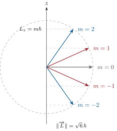
On $\ket{l, m}$ : (a) show $\langle\hat L_x\rangle = \langle\hat L_y\rangle = 0$ ; (b) show $\langle\hat L_x^2\rangle = \langle\hat L_y^2\rangle = \tfrac12[l(l+1) - m^2]\hbar^2$ ; (c) verify the uncertainty relation $\Delta L_x\,\Delta L_y \ge \tfrac\hbar2 |\langle\hat L_z\rangle|$ on the stretched state $m = l$ ; (d) interpret the “cone” picture of the figure in the light of (a) and (b).

Solution

Solution of Exercise 10.9.

(a) $\hat L_x = (\hat L_+ + \hat L_-)/2$ changes $m$ : diagonal elements vanish. (b) By symmetry the two transverse squares are equal, and their sum is $\langle\hat L^2 - \hat L_z^2\rangle$ . (c) At $m = l$ : $\Delta L_x\Delta L_y = l\hbar^2/2 = \tfrac\hbar2 \,l\hbar$ : equality — the stretched state is as aligned as the algebra permits. (d) The cone: sharp $L_z$ , vanishing transverse means, equal transverse spreads — a vector of definite length and projection, democratically smeared in azimuth.

Exercise 10.10 ★★★

Vibration–rotation bands. An infrared vibrational transition ( $\hbar\omega_0$ ) of a diatomic changes $J$ by $\pm1$ simultaneously. (a) Show the absorption lines fall at $h\nu = \hbar\omega_0 + 2B(J+1)$ (the $R$ branch, from $J \to J+1$ ) and $h\nu = \hbar\omega_0 - 2BJ$ (the $P$ branch, $J \to J-1$ ), $J \ge 1$ . (b) Why is there a gap at $\hbar\omega_0$ itself? (c) Sketch the band: two combs flanking a missing central line, each line’s strength following Exercise 10.6. (d) The $15\,\text{µ}\mathrm{m}$ band of Problem 9.1 has exactly this anatomy: what sets its overall width, and hence the “wings” that make added carbon dioxide effective?

Solution

Solution of Exercise 10.10.

(a) Energy bookkeeping with $E_J = BJ(J+1)$ : $J \to J + 1$ adds $2B(J+1)$ ; $J \to J - 1$ subtracts $2BJ$ . (b) $\Delta J = 0$ is forbidden, and the two branches start at $\pm 2B$ : nothing falls at the pure vibrational frequency. (c) Two combs of spacing $2B$ flanking a gap, intensities rising to $J_{\max}$ then falling. (d) The band’s width is the populated extent of the combs, growing as $\sqrt{T}$ : those thermally populated wings are precisely where a saturated greenhouse band keeps absorbing.

Exercise 10.11 ★★★

Finish the algebra. (a) From $\hat J_\mp\hat J_\pm = \hat J^2 - \hat J_z^2 \mp \hbar\hat J_z$ , compute $\|\hat J_\pm\ket{j,m}\|^2$ and the ladder coefficients. (b) Show that if the ladder failed to terminate, some norm would go negative: exhibit the offending state. (c) Conclude that $m_{\max} - m_{\min} = 2j$ must be a non-negative integer and enumerate the allowed $j$ . (d) Where exactly does the argument fail to exclude half-integers — and which additional requirement (single-valuedness on the sphere) excludes them for orbital motion only?

Solution

Solution of Exercise 10.11.

(a) $\|\hat J_\pm\ket{j,m}\|^2 = \bra{j,m}\hat J_\mp\hat J_\pm \ket{j,m} = \hbar^2[j(j+1) - m(m\pm1)]$ . (b) Climbing past $m = j$ would give $j(j+1) - j(j+1) = 0$ then negative norms one step further: the chain must contain the annihilated top state. (c) The top and bottom differ by an integer number of unit steps: $2j \in \mathbb N$ : $j = 0, \tfrac12, 1, \tfrac32, \dots$ (d) The algebra never uses wave functions; only the demand that $\eu^{\iu m\varphi}$ be single-valued on the circle forces integer $m$ — a condition binding orbital motion and leaving intrinsic (spin) angular momenta free to be half-integer.

Exercise 10.12 ★★★

Einstein–de Haas: angular momentum is mechanical. An iron cylinder (radius $a = 1.0\,\mathrm{cm}$ , density $\rho = 7.9 \times 10^{3}\,\mathrm{kg}/\mathrm{m}^{3}$ , $n = 8.5 \times 10^{28}\,\mathrm{atoms}/\mathrm{m}^{3}$ ) hangs from a torsion fibre; reversing its magnetisation flips about one $\hbar$ of angular momentum per atom. (a) By conservation, the rod must recoil: compute the angular momentum per unit volume transferred. (b) With the rod’s moment of inertia $\tfrac12 M a^2$ , show the rod acquires $\omega = 2n\hbar/\rho a^2$ and evaluate it. (c) The 1915 experiment drove the reversal at the fibre’s resonance to accumulate the tiny kicks: estimate the oscillation amplitude after $Q \sim 100$ resonant reversals, taking your $\omega$ per kick. (d) The measured ratio moment/angular-momentum came out twice the orbital prediction $e/2m_{\text{e}}$ : what was that factor of two announcing?

Solution

Solution of Exercise 10.12.

(a) $n\hbar$ per unit volume. (b) $\omega = n\hbar V/(\tfrac12 Ma^2) = 2n\hbar/\rho a^2 = 2 \times 8.5 \times 10^{28} \times 1.055 \times 10^{-34}/ (7900 \times 10^{-4}) \approx 2.3 \times 10^{-5}\,\mathrm{rad}/\mathrm{s}$ — invisible in one shot. (c) Reversing in step with the fibre’s resonance accumulates $\sim Q$ kicks: $\omega \sim 2 \times 10^{-3}\,\mathrm{rad}/\mathrm{s}$ , milliradian swings on a period of seconds — visible with a mirror and a light beam, as Einstein and de Haas saw. (d) The measured gyromagnetic ratio was $e/m_{\text{e}}$ , twice the orbital $e/2m_{\text{e}}$ : iron’s magnetism is not orbital currents but electron spin, whose $g \approx 2$ the next chapters explain.

10.6 Problem: Weighing galaxies at 2.6 millimetres

Problem 10.1

Weekend problem — carbon monoxide, radio astronomy and the cold universe

Most of a galaxy’s star-making matter is cold molecular hydrogen — and it is invisible: H $_2$ , symmetric, has no dipole and no rotational lines at cold-cloud temperatures. Astronomy’s solution is its faithful companion. One CO molecule per $10^{4}$ H $_2$ , with its $115\,\mathrm{GHz}$ ladder, lights up every molecular cloud in the sky. Data: for CO, $B/h = 57.6\,\mathrm{GHz}$ ( $B = 0.238\,\mathrm{meV}$ ); bond length $r_0 = 0.113\,\mathrm{nm}$ ; reduced mass $\mu = 1.14 \times 10^{-26}\,\mathrm{kg}$ ; $k_{\text{B}}T$ at $10\,\mathrm{K}$ is $0.862\,\mathrm{meV}$ .

Part I — The quantum rotor.

From $\hat H = \hat L^2/2I$ , give the energies $E_J$ and their degeneracies.
Verify $B = \hbar^2/2I$ for CO from $r_0$ and $\mu$ .
With the selection rule $\Delta J = \pm1$ , derive the absorption frequencies $\nu_{J+1\leftarrow J} = 2B(J+1)/h$ and list the first three.
Why are the lines equally spaced — and what does a measured spacing hand the astronomer (through $I$ )?
Compute the wavelength of the fundamental line, and explain why observing it needs high, dry sites (what absorbs millimetre waves in our own atmosphere — recall the molecule of Problem 9.1’s neighbour, water)?
The photon of the $1 \to 0$ line carries $\hbar$ of angular momentum: why is $\Delta J = \pm1$ not merely a rule of thumb but a conservation law?

Part II — Why CO and not H $_2$ .

H $_2$ is homonuclear: state why it emits no rotational dipole radiation at all.
H $_2$ is also light: compute the rotational constant of H $_2$ ( $\mu = m_{\text{p}}/2$ , $r_0 = 0.074\,\mathrm{nm}$ ) and its first accessible transition energy; compare with $k_{\text{B}}T$ at $10\,\mathrm{K}$ : even by quadrupole back-doors, could cold H $_2$ radiate?
CO’s first rung costs $2B = 0.48\,\mathrm{meV}$ against $k_{\text{B}}T = 0.86\,\mathrm{meV}$ : is the ladder alive at $10\,\mathrm{K}$ ?
Compute the population ratio $n_1/n_0$ at $10\,\mathrm{K}$ (degeneracy included).
Near which $J$ does the population peak at $10\,\mathrm{K}$ (use $J_{\max} \approx \sqrt{k_{\text{B}}T/2B} - \tfrac12$ )?
Summarise in one sentence the pact of the trade: what CO provides, what must be assumed about the CO-to-H $_2$ ratio.

Part III — Reading the sky.

A cloud’s line arrives at $115.156\,\mathrm{GHz}$ instead of the laboratory $115.271\,\mathrm{GHz}$ : compute the cloud’s velocity along the line of sight, and its direction.
The line is Doppler-broadened by internal motions of $\pm2\,\mathrm{km}/\mathrm{s}$ : compute the linewidth in MHz, and compare with the thermal width expected at $10\,\mathrm{K}$ ( $v_{\text{th}} \sim \sqrt{k_{\text{B}}T/m_{\text{CO}}} \approx 55\,\mathrm{m}/\mathrm{s}$ ): what dominates the broadening?
Mapping the Doppler shift of CO across a spiral galaxy’s disc yields its rotation curve $v(r)$ . The curves stay flat far beyond the visible disc: recall (Year 1 volume, gravitation) what $v(r)$ should do around a centrally concentrated mass, and state what the flatness implies.
The ratio of the $2\to1$ line’s brightness to the $1\to0$ ’s measures level populations: which single physical quantity of the cloud does it deliver?
ALMA resolves CO in galaxies whose light left when the universe was young; the observed frequency of the $1 \to 0$ line from a galaxy at “redshift $z = 1$ ” arrives at half its rest value — at what frequency, and (recalling Example 4.13) what stretched it?
From a measured CO line luminosity astronomers quote cloud masses in solar masses: list the chain of conversions (line photons $\to$ CO count $\to$ H $_2$ mass) and the weakest link.

Part IV — The cold nurseries.

Star-forming cores sit at $10\,\mathrm{K}$ : from Wien’s law their thermal glow peaks near $290\,\text{µ}\mathrm{m}$ — invisible to every optical telescope. In one sentence: why is the rotational ladder the only thermometer and scale such a core offers?
The $J = 1$ level lies $5.5\,\mathrm{K}$ (in temperature units) above the ground state: why does that make the $1\to0$ line an exquisite thermometer precisely in the $10\,\mathrm{K}$ regime (rather than, say, an optical line at $2\,\mathrm{eV}$ $\sim 23\,000\,\mathrm{K}$ )?
Why does a collapsing core eventually stop being visible in CO ( $1\to0$ ) — consider what high density and dust do to the line and its escape.
Molecular clouds also show lines of NH $_3$ , HCN, and dozens more, each with its own $B$ and dipole: what does the richness of this “chemical radio dial” let astronomers disentangle?
The whole sky glows at $2.7\,\mathrm{K}$ (the cosmic microwave background): what happens to the contrast of a cloud’s CO lines as the cloud’s own temperature approaches $2.7\,\mathrm{K}$ , and why is that a hard floor for this thermometer?
A millimetre dish must hold its shape to about $\lambda/20$ : compute that tolerance at $115\,\mathrm{GHz}$ , and compare with the tolerance an optical mirror ( $500\,\mathrm{nm}$ ) must meet — why could ALMA’s twelve-metre dishes be built in the open air?
Summarise the named result: a ladder $BJ(J+1)$ with $B/h = 57.6\,\mathrm{GHz}$ , populated at ten kelvin and read at $2.6\,\mathrm{mm}$ , is how the mass, temperature, velocity and rotation of the cold universe — and the evidence for dark matter around spiral galaxies — are measured.

Solution

Solution of Problem 10.1.

1. $E_J = BJ(J+1)$ , degeneracy $2J + 1$ . 2. $I = \mu r_0^2 = 1.46 \times 10^{-46}\,\mathrm{kg}\,\mathrm{m}^{2}$ : $B = \hbar^2/2I = 3.8 \times 10^{-23}\,\mathrm{J}$ , i.e. $B/h = 57.7\,\mathrm{GHz}$ — the measured constant. 3. $115$ , $231$ , $346\,\mathrm{GHz}$ . 4. $E_{J+1} - E_J = 2B(J+1)$ grows linearly: consecutive lines differ by the constant $2B$ . The spacing gives $I$ , hence the bond length — structural chemistry by radio. 5. $\lambda = c/\nu = 2.6\,\mathrm{mm}$ . Atmospheric water vapour absorbs millimetre waves greedily; hence Atacama, Mauna Kea, the South Pole — high, cold, dry. 6. The photon is a spin- $1$ particle carrying $\hbar$ : total angular momentum conservation obliges the molecule’s $J$ to change by one unit. 7. Its charge distribution is symmetric at every rotation angle: no oscillating dipole, no dipole line — perfect camouflage. 8. $B_{\text{H}_2} = \hbar^2/2\mu r_0^2 \approx 7.6\,\mathrm{meV}$ ; the symmetric molecule’s weak quadrupole transitions require $\Delta J = 2$ , costing $6B \approx 46\,\mathrm{meV}$ — fifty times $k_{\text{B}}T$ at $10\,\mathrm{K}$ : cold hydrogen cannot radiate at all. 9. $2B = 0.48\,\mathrm{meV} < k_{\text{B}}T = 0.86\,\mathrm{meV}$ : collisions keep the first rungs populated — the ladder works exactly where the clouds live. 10. $n_1/n_0 = 3\,\eu^{-0.478/0.862} = 1.7$ : the emitting level is well stocked. 11. $J_{\max} \approx \sqrt{0.86/0.48} - 0.5 \approx 0.8$ : the population peaks at $J = 1$ . 12. CO delivers the photons; converting them to total gas mass rests on an assumed CO-to-H $_2$ abundance — luminous messenger, calibrated ransom. 13. $\Delta\nu = 115\,\mathrm{MHz}$ : $v = c\,\Delta\nu/\nu \approx 300\,\mathrm{km}/\mathrm{s}$ , receding (frequency lowered) — galactic orbital speeds. 14. $\pm2\,\mathrm{km}/\mathrm{s}$ spans $1.5\,\mathrm{MHz}$ ; thermal motion at $10\,\mathrm{K}$ gives only $\sim40\,\mathrm{kHz}$ : the width is turbulence, not temperature — linewidths map a cloud’s internal weather. 15. Around a central mass $v \propto 1/\sqrt r$ should fall (Kepler); the measured flatness means the enclosed mass keeps growing with radius — invisible matter enveloping the luminous disc: dark matter. 16. The ratio of populations, i.e. the excitation temperature of the gas. 17. At $57.6\,\mathrm{GHz}$ : cosmic expansion has doubled every wavelength in flight — the cosmological redshift the last chapter of this book returns to. 18. Photon flux $\to$ CO luminosity (distance needed) $\to$ CO count (excitation model) $\to$ H $_2$ mass (the CO-to-H $_2$ “X-factor”: the weakest link, calibrated locally and exported cautiously). 19. A $10\,\mathrm{K}$ core emits nothing an optical telescope can see; its rotational lines are simultaneously its only thermometer, speedometer and scale. 20. A thermometer is sensitive where level spacing $\sim k_{\text{B}}T$ : $5.5\,\mathrm{K}$ spacing responds strongly across $5$ – $50$ K, while a $2\,\mathrm{eV}$ optical level would be populated by nothing at all. 21. The line saturates (optically thick) and, worse, CO freezes out onto dust grains in the densest, coldest gas: astronomers switch to rarer isotopologues ( $^{13}$ CO, C $^{18}$ O) and other molecules. 22. Each species needs its own density and temperature to shine: together they tomograph the cloud — outer envelopes in CO, dense cores in NH $_3$ and HCN. 23. A line is seen in contrast against the cosmic background; as the gas temperature approaches $2.7\,\mathrm{K}$ its excitation equilibrates with the background and the contrast vanishes: no colder cloud can be read this way. 24. $\lambda/20 = 130\,\text{µ}\mathrm{m}$ against $25\,\mathrm{nm}$ for optical work: five thousand times more forgiving — which is why twelve-metre millimetre dishes stand in the open desert while optical mirrors live in domes. 25. A ladder $BJ(J+1)$ with $B/h = 57.6\,\mathrm{GHz}$ , alive at ten kelvin and read at $2.6\,\mathrm{mm}$ , measures the mass, temperature, turbulence and rotation of the cold universe — and its flat rotation curves are a standing exhibit for dark matter.

Terms defined in this chapter

Angular momentum operators

See all 431 terms in the glossary