University Physics — Year 3 · Bachelor Year 3

8The Formalism of Quantum Mechanics

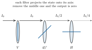
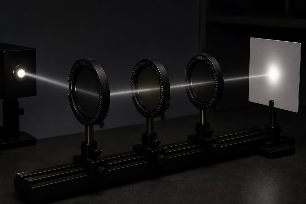
Take three polarizing filters. Two of them, crossed at $90^\circ$ , block light completely; slide the third between them at $45^\circ$ and light comes through — adding an obstacle opens the way. No picture of filters as sieves survives this experiment; what does survive is linear algebra: the polarization of a photon is a vector, each filter measures it along an axis and projects it, and the probabilities are squared components. This chapter installs that algebra as the actual foundation of quantum mechanics. The wave functions of the previous chapters were one concrete costume of a more abstract body: states are vectors in a Hilbert space, observables are Hermitian operators, measured values are eigenvalues, probabilities are squared scalar products, and evolution is generated by the Hamiltonian. Five postulates, all of them already at work in everything we have computed — and, once stated cleanly, powerful enough to handle systems no wave on a line can describe: the photon’s polarization, the electron’s spin, and the neutrinos whose identity oscillates across the Earth.

8.1 States are vectors

Definition 8.1 (State space, kets and brackets)

The states of a quantum system form a complex vector space with an inner product — a Hilbert space $\mathcal H$ (the mathematics is developed in the Year 3 mathematics volume). A state is a vector, written as a ket $\ket\psi$ , normalised: $\braket\psi\psi = 1$ . The inner product of two states is the complex number $\braket\varphi\psi$ , conjugate-linear in the first slot, with $\braket\varphi\psi = \braket\psi\varphi^*$ . In an orthonormal basis $\{\ket{e_i}\}$ ,

\ket\psi = \sum_i c_i\ket{e_i} , \qquad c_i = \braket{e_i}\psi , \qquad \sum_i|c_i|^2 = 1 .

The wave function of the previous chapters is the family of components of $\ket\psi$ along position: $\psi(x) = \braket{x}{\psi}$ ; nothing is lost, and systems with finite state spaces — undreamable as waves — become describable.

Example 8.2 (The photon’s polarization: a two-dimensional world)

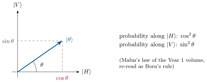
A photon heading down the $z$ axis carries a polarization state in a two-dimensional Hilbert space, with basis $\ket H$ (horizontal) and $\ket V$ (vertical). Light polarized at angle $\theta$ is the superposition

\ket\theta = \cos\theta\,\ket H + \sin\theta\,\ket V ,

and circular polarization is the complex combination $(\ket H \pm \iu\ket V)/\sqrt2$ : the coefficients being complex is not decoration but physics. Every quantum two-level system — spin, the ammonia molecule, a superconducting qubit — is this same vector space in different clothing.

A polarization state as a vector: its squared components on an analyser’s basis are the outcome probabilities — geometry become probability.

8.2 Observables are operators

Definition 8.3 (Observables)

An observable is a linear operator $\hat A$ on $\mathcal H$ that is Hermitian: $\braket{\varphi}{\hat A\psi} = \braket{\hat A\varphi}{\psi}$ for all states (in matrix language, $A = A^{*\top}$ ). Its eigenvectors and eigenvalues, $\hat A\ket{a} = a\ket{a}$ , carry the physics: the $a$ are the possible measured values. Familiar cases: position ( $\hat x$ : multiplication by $x$ ), momentum ( $\hat p = -\iu\hbar\,\dd/\dd x$ ), energy ( $\hat H = \hat p^2/2m + V(\hat x)$ ) — and, in two dimensions, any Hermitian $2\times2$ matrix.

Theorem 8.4 (Why Hermitian)

A Hermitian operator has real eigenvalues, and eigenvectors with distinct eigenvalues are orthogonal; on the spaces of this book its eigenvectors form an orthonormal basis of $\mathcal H$ (the spectral theorem, proved in finite dimension in the Year 2 mathematics volume; for the unbounded operators $\hat x$ , $\hat p$ , $\hat H$ the full statement belongs to Year 3 spectral theory and is admitted). Measured values must be real and distinguishable outcomes must be orthogonal: Hermiticity is exactly the condition that an operator can represent a measurement.

Partial proof. $a\braket aa = \braket{a}{\hat Aa} = \braket{\hat Aa}{a} = a^*\braket aa$ : $a$ real. For $\hat A\ket a = a\ket a$ , $\hat A\ket b = b\ket b$ : $a\braket ba = \braket{b}{\hat Aa} = \braket{\hat Ab}{a} = b\braket ba$ , so $(a - b)\braket ba = 0$ . ∎

Example 8.5 (A two-level observable)

On the polarization space, in the $(\ket H, \ket V)$ basis, consider

\hat A = \begin{pmatrix} 0 & 1\\ 1 & 0\end{pmatrix} :

Hermitian; eigenvalues $\pm1$ ; eigenvectors $(\ket H \pm \ket V)/\sqrt2$ — the polarizations at $\pm45^\circ$ . Measuring $\hat A$ means asking “diagonal or antidiagonal?”, and the eigenbasis is the pair of questions’ answers. Every $45^\circ$ polarizer in the opening experiment is this matrix in glass.

8.3 The postulates

Theorem 8.6 (The rules of quantum mechanics)

(P1) A system’s state is a normalised ket $\ket\psi$ in its Hilbert space. (P2) Every measurable quantity is a Hermitian operator $\hat A$ . (P3) The only possible results of measuring $\hat A$ are its eigenvalues. (P4) On a state $\ket\psi$ , the result $a$ occurs with probability $\mathcal P(a) = |\braket a\psi|^2$ (Born’s rule; for a degenerate eigenvalue, sum the squared components over its eigenspace). The mean of many trials is $\langle\hat A\rangle = \bra\psi\hat A\ket\psi$ . (P5) Immediately after a measurement giving $a$ , the state is the (normalised) projection of $\ket\psi$ onto the $a$ eigenspace — the collapse: measurement is an interaction that leaves the system in the state matching its own answer. (P6) Between measurements, the state evolves unitarily under the Schrödinger equation $\iu\hbar\,\dfrac{\dd}{\dd t}\ket{\psi(t)} = \hat H\ket{\psi(t)}$ .

Proof. Admitted at this level. ∎

Example 8.7 (The three polarizers, computed)

Vertical light meets a $90^\circ$ -crossed analyser: $|\braket HV|^2 = 0$ — extinction. Insert a $45^\circ$ polarizer: the state $\ket V$ passes it with probability $|\braket{45^\circ}{V}|^2 = \tfrac12$ and collapses to $\ket{45^\circ}$ (P5); that state then passes the horizontal analyser with probability $|\braket{H}{45^\circ}|^2 = \tfrac12$ . Net transmission $\tfrac14$ instead of zero: the middle filter does not “open a hole” — it performs a measurement, and the collapse re-prepares the photon. No classical sieve does this; a projection does nothing else.

The three-polarizer experiment as three successive measurements: project, collapse, project again. An added filter increases the transmitted light — impossible for sieves, automatic for projections.

Remark 8.8 (What the collapse does not allow)

Collapse is instantaneous in the formalism, and quantum correlations between distant particles are real and measured — but no message rides on them: the outcomes at one detector, read alone, are indistinguishable from coin flips whatever is done far away. Quantum randomness is also irreducible: Born’s rule gives probabilities even when the state is known completely — there is nothing more to know. Both statements are theorems of the formalism, tested to high precision; unease about them is respectable and has driven a century of experiments, every one of which quantum mechanics has won.

8.4 Commutators and uncertainty

Definition 8.9 (Commutator; compatible observables)

The commutator of two operators is $[\hat A, \hat B] = \hat A\hat B - \hat B\hat A$ . The founding example, from $\hat p = -\iu\hbar\,\dd/\dd x$ :

[\hat x, \hat p] = \iu\hbar .

Two observables are compatible when $[\hat A, \hat B] = 0$ : they then admit a common eigenbasis and can be known simultaneously; measuring one does not disturb a state sharp in the other. A set of commuting observables whose common eigenbasis is unique (a CSCO) is what “completely labelling a state” means — the labels $(n_1, n_2, n_3)$ of the box were exactly this.

Theorem 8.10 (The uncertainty relation, in general)

In any state, the standard deviations of two observables obey

\Delta A\;\Delta B \ \ge\ \tfrac12\,\big|\langle[\hat A, \hat B]\rangle\big| .

For $\hat x$ and $\hat p$ : $\Delta x\,\Delta p \ge \hbar/2$ — Heisenberg’s relation, now a theorem of linear algebra rather than a heuristic. Incompatibility is quantitative: the commutator’s size sets the floor under joint sharpness.

Partial proof. Let $\hat\alpha = \hat A - \langle A\rangle$ , $\hat\beta = \hat B - \langle B\rangle$ . The Cauchy–Schwarz inequality of the Year 3 mathematics volume gives $\Delta A^2\Delta B^2 = \|\hat\alpha\psi\|^2\|\hat\beta\psi\|^2 \ge |\braket{\hat\alpha\psi}{\hat\beta\psi}|^2$ ; the imaginary part of that product is $\tfrac1{2\iu}\langle[\hat A, \hat B]\rangle$ , and $|z|^2 \ge (\operatorname{Im}z)^2$ . ∎

Remark 8.11 (The classical shadow)

Divide by $\iu\hbar$ and let $\hbar \to 0$ : commutators become the Poisson brackets of Chapter 2, $\{x, p\} = 1$ echoing $[\hat x, \hat p] = \iu\hbar$ , and the angular-momentum brackets computed there will return as commutators, unchanged, in Chapter 10. Dirac’s rule — classical bracket times $\iu\hbar$ — is how the skeleton of mechanics survived the revolution.

8.5 Evolution and conservation

Proposition 8.12 (Evolution of averages; conserved quantities)

For an observable without explicit time dependence,

\frac{\dd\langle\hat A\rangle}{\dd t} = \frac{\iu}{\hbar}\,\big\langle[\hat H, \hat A]\big\rangle .

An observable commuting with the Hamiltonian is conserved — its probabilities, not merely its mean, are frozen; symmetries again deliver conservation laws, now as commutation. Stationary states are the eigenvectors of $\hat H$ , evolving only by the phase $\eu^{-\iu Et/\hbar}$ ; a superposition of two levels beats at the Bohr frequency $(E_2 - E_1)/h$ , as the Year 2 volume’s wells already showed.

Proof. Differentiate $\bra\psi\hat A\ket\psi$ and insert P6 and its conjugate:

\frac{\dd\langle\hat A\rangle}{\dd t} = \frac{\iu}{\hbar}\bra\psi\hat H\hat A\ket\psi - \frac{\iu}{\hbar}\bra\psi\hat A\hat H\ket\psi = \frac{\iu}{\hbar}\,\langle[\hat H, \hat A]\rangle . \qedhere

∎

Method 8.13 (Matrix quantum mechanics)

For any finite-level problem: (1) choose a basis suited to the question (the analyser’s axes, the energy eigenstates); (2) write states as column vectors, observables as Hermitian matrices; (3) diagonalise what is measured — eigenvalues are the outcomes, squared components the probabilities; (4) evolve energy eigenstates by phases $\eu^{-\iu E_it/\hbar}$ and re-express in the measurement basis; (5) after a measurement, restart from the projected state. The whole of Problem 8.1 is this recipe run on a two-level universe.

Three polarisers on a bench: each is a measurement, projecting the light’s state onto an axis. Cross two and nothing passes; slip a third between them at an angle and light returns — the postulates of this chapter, performed on a table.

8.6 Exercises

Exercise 8.1 ★

In an orthonormal basis $(\ket1, \ket2)$ , let $\ket\psi = (2\ket1 + \iu\ket2)/\sqrt5$ and $\ket\varphi = (\ket1 - \ket2)/\sqrt2$ . (a) Check the normalisations. (b) Compute $\braket\varphi\psi$ and $\braket\psi\varphi$ . (c) The probability of finding $\ket\psi$ in the state $\ket\varphi$ . (d) Construct the state orthogonal to $\ket\psi$ (up to phase).

Solution

Solution of Exercise 8.1.

(a) $(4 + 1)/5 = 1$ and $(1 + 1)/2 = 1$ . (b) $\braket\varphi\psi = (2 - \iu)/\sqrt{10}$ ; $\braket\psi\varphi = (2 + \iu)/\sqrt{10}$ : conjugates. (c) $|(2 - \iu)|^2/10 = 1/2$ . (d) Solve $\braket\psi\chi = 0$ : $\ket\chi = (\ket1 - 2\iu\ket2)/\sqrt5$ .

Exercise 8.2 ★

Which of these matrices are Hermitian, and what are the eigenvalues and normalised eigenvectors of those that are?

\begin{pmatrix}0 & 1\\ 1 & 0\end{pmatrix} , \quad \begin{pmatrix}0 & -\iu\\ \iu & 0\end{pmatrix} , \quad \begin{pmatrix}1 & 1\\ -1 & 1\end{pmatrix} , \quad \begin{pmatrix}2 & 1-\iu\\ 1+\iu & 3\end{pmatrix} .

Solution

Solution of Exercise 8.2.

First: Hermitian; $\pm1$ with $(\ket1 \pm \ket2)/\sqrt2$ . Second: Hermitian; $\pm1$ with $(\ket1 \pm \iu\ket2)/\sqrt2$ . Third: not Hermitian (the transpose-conjugate differs). Fourth: Hermitian; $\lambda^2 - 5\lambda + 4 = 0$ gives $1$ and $4$ , with eigenvectors $\big({-(1 - \iu)}\ket1 + \ket2\big)/\sqrt3$ and $\big(\ket1 + (1 + \iu)\ket2\big)/\sqrt3$ .

Exercise 8.3 ★

Light polarized at angle $\alpha$ meets an analyser at angle $\beta$ . (a) Write both states in the $(\ket H, \ket V)$ basis and compute the transmission probability. (b) Recover Malus’s law. (c) For a stream of $N$ photons, what is the variance of the transmitted number? (d) Circular light $(\ket H + \iu\ket V)/\sqrt2$ on a linear analyser at any angle: transmission? Explain the answer’s independence of the angle.

Solution

Solution of Exercise 8.3.

(a) $\braket\beta\alpha = \cos\beta\cos\alpha + \sin\beta\sin\alpha = \cos(\beta - \alpha)$ : probability $\cos^2(\beta - \alpha)$ . (b) Intensity $\propto$ photon number: Malus. (c) Each photon is an independent trial: variance $N\mathcal P(1 - \mathcal P)$ — the noise itself certifies photons. (d) $|\cos\beta + \iu\sin\beta|^2/2 = 1/2$ for every $\beta$ : circular light singles out no transverse axis.

Exercise 8.4 ★

(a) Prove $[\hat x, \hat p] = \iu\hbar$ by acting on a test function. (b) Compute $[\hat x^2, \hat p]$ and $[\hat x, \hat p^2]$ . (c) Show $[\hat A, \hat B\hat C] = [\hat A, \hat B]\hat C + \hat B[\hat A, \hat C]$ . (d) Deduce $[\hat x, \hat p^n] = \iu\hbar\,n\hat p^{n-1}$ and interpret: which classical operation does $[\hat x, \cdot\,]$ mimic?

Solution

Solution of Exercise 8.4.

(a) $(\hat x\hat p - \hat p\hat x)f = -\iu\hbar(xf' - (xf)') = \iu\hbar f$ . (b) $[\hat x^2, \hat p] = 2\iu\hbar\hat x$ ; $[\hat x, \hat p^2] = 2\iu\hbar\hat p$ . (c) Add and subtract $\hat B\hat A \hat C$ . (d) Induction with (c): $\iu\hbar\,n\hat p^{n-1}$ — $[\hat x, \cdot]$ acts as $\iu\hbar\,\partial/\partial p$ , the quantum shadow of the Poisson bracket with $x$ .

Exercise 8.5 ★★

Sequential measurements. A photon starts as $\ket V$ . (a) It meets polarizers at $45^\circ$ then $0^\circ$ (horizontal): compute the probability of surviving both, with the intermediate collapse made explicit. (b) Replace the middle polarizer by ones at $30^\circ$ , $60^\circ$ : transmission? (c) $N - 1$ intermediate polarizers stepping by $90^\circ/N$ : show the survival probability is $\cos^{2N}(\pi/2N)$ and evaluate for $N = 2, 5, 20$ . (d) The limit $N \to \infty$ rotates the polarization with no loss: comment (this “quantum Zeno” rotation is used on real qubits).

Solution

Solution of Exercise 8.5.

(a) $|\braket{45^\circ}{V}|^2 = \tfrac12$ , collapse, then $|\braket{H}{45^\circ}|^2 = \tfrac12$ : total $\tfrac14$ . (b) Taking them in the order $60^\circ$ , $30^\circ$ (three steps of $30^\circ$ ): $(\cos^230^\circ)^3 = 27/64 \approx 0.42$ . (c) Each step of $\pi/2N$ passes with $\cos^2(\pi/2N)$ : survival $[\cos^2(\pi/2N)]^N = 0.25$ , $0.60$ , $0.88$ for $N = 2, 5, 20$ . (d) As $N \to \infty$ the survival tends to $1$ : many gentle measurements steer the state through $90^\circ$ without loss — measurement used as a steering wheel.

Exercise 8.6 ★★

On the two-level space, $\hat A = \begin{pmatrix}0&1\\1&0 \end{pmatrix}$ , $\hat B = \begin{pmatrix}1&0\\0&-1\end{pmatrix}$ . (a) Compute $[\hat A, \hat B]$ : compatible? (b) The state is $\ket1$ : give the outcome statistics of measuring $\hat B$ , then of measuring $\hat A$ after a $\hat B$ measurement gave $+1$ . (c) Measure $\hat A$ first (outcome $+1$ ), then $\hat B$ , then $\hat A$ again: with what probability does the final $\hat A$ contradict the first? (d) What would zero commutator have implied for (c)?

Solution

Solution of Exercise 8.6.

(a) $[\hat A, \hat B] = \begin{pmatrix}0 & -2\\ 2 & 0\end{pmatrix} \neq 0$ : incompatible. (b) $\hat B$ on $\ket1$ : $+1$ with certainty, no collapse needed; $\hat A$ then gives $\pm1$ with probability $\tfrac12$ each. (c) After $\hat A \to +1$ the state is $(\ket1 + \ket2)/\sqrt2$ ; $\hat B$ collapses it to $\ket1$ or $\ket2$ (each $\tfrac12$ ); either way the final $\hat A$ gives $\pm1$ with probability $\tfrac12$ : contradiction with probability $\tfrac12$ . (d) Commuting observables share eigenstates: the middle measurement would not disturb, and the repetition would agree with certainty.

Exercise 8.7 ★★

(a) For the Gaussian state of Exercise 7.1 restricted to one dimension, compute $\Delta x$ and $\Delta p$ (use the Fourier pair or integrate) and verify equality in Heisenberg’s relation. (b) Which states saturate the general uncertainty theorem (state the condition from the Cauchy–Schwarz equality case)? (c) An electron confined to $\Delta x = 0.1\,\mathrm{nm}$ : minimum kinetic energy scale? (d) Same for a marble ( $10\,\mathrm{g}$ ) localised to a micron: conclude.

Solution

Solution of Exercise 8.7.

(a) $\Delta x = \sigma$ and $\Delta p = \hbar/2\sigma$ (the Fourier transform of a Gaussian of width $\sigma$ has width $1/2\sigma$ in $k$ ): product exactly $\hbar/2$ . (b) Equality in Cauchy–Schwarz: $\hat\beta\ket\psi \propto \hat\alpha\ket\psi$ with purely imaginary ratio — for $x, p$ this differential equation has Gaussian solutions only. (c) $\Delta p \ge 5.3 \times 10^{-25}\,\mathrm{kg}\,\mathrm{m}/\mathrm{s}$ : $E \sim \Delta p^2/2m_{\text{e}} \approx 1\,\mathrm{eV}$ — atoms are electron-volt machines because they are ångström boxes. (d) $\Delta v \ge 5 \times 10^{-27}\,\mathrm{m}/\mathrm{s}$ : nothing, ever.

Exercise 8.8 ★★

(a) From Proposition 8.12, recover Ehrenfest’s pair for $\hat x$ and $\hat p$ with $\hat H = \hat p^2/2m + V$ . (b) Show that parity $\hat\Pi$ ( $\hat\Pi\psi(x) = \psi(-x)$ ) is Hermitian, squares to the identity, and has eigenvalues $\pm1$ . (c) Show $[\hat H, \hat\Pi] = 0$ for a symmetric potential and conclude that non-degenerate levels have definite parity. (d) Which observed fact about the levels of a symmetric double well does this explain (recall the ammonia doublet of the Year 2 volume)?

Solution

Solution of Exercise 8.8.

(a) $[\hat H, \hat x] = -\iu\hbar\hat p/m$ and $[\hat H, \hat p] = \iu\hbar V'(\hat x)$ give $\dd\langle x\rangle/\dd t = \langle p\rangle/m$ , $\dd\langle p\rangle/\dd t = -\langle V'\rangle$ . (b) Change of variable in the inner product shows Hermiticity; $\hat\Pi^2 = \mathbb 1$ forces eigenvalues $\pm1$ . (c) $V(-x) = V(x)$ makes $\hat H$ parity-blind; a non-degenerate eigenstate must then be an eigenstate of $\hat\Pi$ too: even or odd. (d) The symmetric double well’s near-degenerate doublet: one even, one odd state — the ammonia inversion pair, split by tunnelling, radiating at $24\,\mathrm{GHz}$ .

Exercise 8.9 ★★

A CSCO at work. In the square two-dimensional box, the level $E \propto 5$ is spanned by $\ket{1,2}$ and $\ket{2,1}$ . (a) Show energy alone does not label states. (b) Let $\hat S$ exchange $x \leftrightarrow y$ : show $\hat S$ is Hermitian, commutes with $\hat H$ , and find its eigenstates within the level. (c) Verify that the pair $(\hat H, \hat S)$ labels every state of this level uniquely. (d) Give the general moral: degeneracy means the labelling set was not yet complete, and symmetry supplies the missing label.

Solution

Solution of Exercise 8.9.

(a) Both states share $E$ : announcing the energy leaves two possibilities. (b) $\hat S$ swaps the labels: Hermitian, squares to identity, commutes with the symmetric $\hat H$ ; within the level its eigenstates are $(\ket{1,2} \pm \ket{2,1})/\sqrt2$ with eigenvalues $\pm1$ . (c) $(E, +)$ and $(E, -)$ : unique labels. (d) A degeneracy is an incomplete address; the symmetry that causes it also provides the missing digit.

Exercise 8.10 ★★★

Energy–time uncertainty, honestly. For any observable $\hat A$ , define the evolution time $\tau_A = \Delta A\,/\,|\dd\langle\hat A\rangle/\dd t|$ — the time for the mean to move by one standard deviation. (a) From Theorem 8.10 and Proposition 8.12, prove $\Delta E\;\tau_A \ge \hbar/2$ . (b) Why is this not an uncertainty between two observables (what is time, in the formalism)? (c) Apply to an excited atomic state of lifetime $10\,\mathrm{ns}$ : linewidth. (d) Apply to your wristwatch: how sharp can the energy of a system be if something in it visibly changes every second?

Solution

Solution of Exercise 8.10.

(a) $\Delta E\,\Delta A \ge \tfrac12|\langle[\hat H, \hat A]\rangle| = \tfrac\hbar2|\dd\langle A\rangle/\dd t|$ ; divide. (b) Time is a parameter of the theory, not an operator: the relation bounds how fast anything measurable can evolve, given the energy spread. (c) $\Delta E \sim \hbar/2\tau = 3.3 \times 10^{-8}\,\mathrm{eV}$ : a natural linewidth of a few megahertz. (d) A visible change per second demands only $\Delta E \gtrsim 5 \times 10^{-35}\,\mathrm{J}$ — for macroscopic energies, no constraint at all: watches may tick.

Exercise 8.11 ★★★

Proof of the uncertainty theorem. With $\hat\alpha, \hat\beta$ as in the text: (a) justify $\Delta A^2 = \|\hat\alpha\ket\psi\|^2$ using Hermiticity; (b) apply Cauchy–Schwarz and split $\braket{\hat\alpha\psi}{\hat\beta\psi}$ into Hermitian and anti-Hermitian parts, identifying them with the anticommutator and commutator averages; (c) conclude, and state when equality holds; (d) show that for $[\hat A, \hat B] = \iu\hbar$ no state can be an eigenvector of either observable while keeping both deviations finite — and reconcile with plane waves.

Solution

Solution of Exercise 8.11.

(a) $\|\hat\alpha\psi\|^2 = \braket{\psi}{\hat\alpha^2\psi} = \Delta A^2$ by Hermiticity of $\hat\alpha$ . (b) $\braket{\hat\alpha \psi}{\hat\beta\psi} = \tfrac12\langle\{\hat\alpha, \hat\beta\}\rangle + \tfrac12\langle[\hat A, \hat B]\rangle$ : the first term is real (Hermitian part), the second purely imaginary. (c) $|z|^2 \ge (\operatorname{Im}z)^2$ gives the theorem; equality needs proportional vectors and vanishing anticommutator average. (d) An eigenstate of $\hat A$ has $\Delta A = 0$ , forcing $0 \ge \hbar/2$ : impossible for normalisable states. Plane waves “achieve” it only by being non-normalisable idealisations outside the Hilbert space.

Exercise 8.12 ★★★

The watched pot. A two-level system starts in $\ket1$ and its Hamiltonian drives Rabi-like oscillation: after time $t$ the state is $\cos(\omega t)\ket1 + \sin(\omega t)\ket2$ (take this as given). (a) With no measurement, when is the transfer to $\ket2$ complete? (b) Measure “which state?” at times $T/N, 2T/N, \dots$ with $T = \pi/2\omega$ : show the probability of finding the system still in $\ket1$ at every check is $[\cos^2(\pi/2N)]^N$ . (c) Evaluate for $N = 1, 4, 20, 100$ and show it tends to $1$ : frequent observation freezes the evolution (the quantum Zeno effect, observed with trapped ions in 1990). (d) Explain in one sentence which postulate does the freezing.

Solution

Solution of Exercise 8.12.

(a) At $\omega t = \pi/2$ , i.e. $t = T$ . (b) At each check the state has rotated by $\pi/2N$ ; it is found in $\ket1$ with $\cos^2(\pi/2N)$ and collapses back to $\ket1$ ; the checks are independent, so the product. (c) $0$ , $0.53$ , $0.88$ , $0.98$ : watched closely enough, the pot never boils. (d) The projection postulate (P5): each observation resets the evolution to its starting line.

The 1927 Solvay conference (photograph by Benjamin Couprie, public domain): the people who built this chapter’s postulates, in one room — and still arguing, that very week, about what measurement means.

8.7 Problem: Neutrinos change costume mid-flight

Problem 8.1

Weekend problem — two-level oscillations across the Earth

Neutrinos are born in nuclear reactions as flavour states — electron-neutrino $\ket{\nu_e}$ or muon-neutrino $\ket{\nu_\mu}$ — but they propagate as energy (mass) eigenstates $\ket{\nu_1}, \ket{\nu_2}$ . The two bases do not coincide: they are rotated by a mixing angle $\theta$ ,

\ket{\nu_e} = \cos\theta\,\ket{\nu_1} + \sin\theta\,\ket{\nu_2} , \qquad \ket{\nu_\mu} = -\sin\theta\,\ket{\nu_1} + \cos\theta\,\ket{\nu_2} .

The discovery that neutrinos therefore oscillate between flavours in flight — hence have mass — earned the 2015 Nobel Prize. This problem derives the effect with nothing beyond this chapter. An ultrarelativistic neutrino of momentum $p$ and mass $m_i$ has energy $E_i \approx pc + m_i^2c^4/2pc \approx E + m_i^2c^4/2E$ .

Part I — The formalism set up.

Check that $(\ket{\nu_1}, \ket{\nu_2})$ orthonormal makes $(\ket{\nu_e}, \ket{\nu_\mu})$ orthonormal too.
Why must the propagation basis be the energy eigenbasis, whatever basis the neutrino was born in? (Which postulate governs free flight?)
A muon-neutrino is born at $t = 0$ . Write $\ket{\psi(0)}$ in the mass basis.
Write $\ket{\psi(t)}$ , each mass component carrying its phase $\eu^{-\iu E_it/\hbar}$ .
Show that a global phase is irrelevant and factor out $\eu^{-\iu E_1t/\hbar}$ : only the relative phase $\Delta\phi = (E_2 - E_1)t/\hbar$ drives the physics.
Express $E_2 - E_1$ in terms of $\Delta m^2 = m_2^2 - m_1^2$ and $E$ , for ultrarelativistic neutrinos.

Part II — The oscillation formula.

Compute the amplitude $\braket{\nu_e}{\psi(t)}$ .
Show the appearance probability is

$\mathcal P_{\nu_\mu \to \nu_e}(t) = \sin^2(2\theta)\,\sin^2\Big(\frac{\Delta\phi}{2}\Big) .$

(Use $2\sin\theta\cos\theta = \sin2\theta$ .)
Check the two sanity limits: $\theta = 0$ and $m_1 = m_2$ . What does any observed oscillation therefore prove?
With $t \approx L/c$ , show

$\mathcal P = \sin^2(2\theta)\, \sin^2\Big(\frac{\Delta m^2c^4}{4\hbar c}\,\frac{L}{E}\Big) ,$

and define the oscillation length $L_{\text{osc}} = 4\pi\hbar cE/\Delta m^2c^4$ .
Show the survival probability $\mathcal P_{\nu_\mu \to \nu_\mu} = 1 - \mathcal P_{\nu_\mu\to\nu_e}$ : where has unitarity been used?
Why does the oscillation measure only $\Delta m^2$ , never the masses themselves?

Part III — Reading the experiments. Atmospheric muon-neutrinos ( $E \approx 1\,\mathrm{GeV}$ ) rain on a detector from above ( $L \approx 15\,\mathrm{km}$ ) and from below, through the Earth ( $L \approx 12\,800\,\mathrm{km}$ ). Super-Kamiokande (1998) found the from-below flux halved, the from-above flux intact.

Using $\hbar c = 197\,\mathrm{MeV}\,\mathrm{fm}$ , show the handy form $\dfrac{\Delta m^2c^4\,L}{4\hbar cE} = 1.27\, \dfrac{\Delta m^2c^4\,[\mathrm{eV}^{2}]\ L\,[\mathrm{km}]} {E\,[\mathrm{GeV}]}$ .
If the oscillation is to be well developed at $L = 12\,800\,\mathrm{km}$ but negligible at $15\,\mathrm{km}$ for $E = 1\,\mathrm{GeV}$ , bracket $\Delta m^2c^4$ roughly.
The measured value is $\Delta m^2c^4 \approx 2.5 \times 10^{-3}\,\mathrm{eV}^{2}$ : compute the oscillation length at $1\,\mathrm{GeV}$ and check it against both baselines.
The from-below suppression is close to $1/2$ , not to $0$ : show that averaging $\sin^2$ over many oscillation lengths (and over energies) gives $\tfrac12\sin^22\theta$ , and deduce that the atmospheric mixing is nearly maximal ( $\theta \approx 45^\circ$ ).
What does $\Delta m^2c^4 = 2.5 \times 10^{-3}\,\mathrm{eV}^{2}$ give for the heavier mass alone if the lighter is negligible — and compare that with the electron’s mass: how oddly light are neutrinos?
Reactor antineutrinos have $E \approx 4\,\mathrm{MeV}$ . Using the same $1.27$ formula, show that a baseline of one to two kilometres is tuned to the $2.5 \times 10^{-3}\,\mathrm{eV}^{2}$ splitting (the Daya Bay experiment), while $L \approx 180\,\mathrm{km}$ (KamLAND) is tuned to the smaller “solar” splitting $7.5 \times 10^{-5}\,\mathrm{eV}^{2}$ — verify both numerically.

Part IV — What it means.

The Sun emits $\nu_e$ ; for decades detectors counted only a third of the prediction. Explain the “solar neutrino problem” and its resolution in one sentence each.
Why did oscillations force the conclusion that neutrinos have mass, against the Standard Model’s original bookkeeping?
A quantum system maintaining phase coherence over $12800$ kilometres: what does this say about how weakly neutrinos interact, and why the detector must be enormous?
Flavour is an observable: why does its operator fail to commute with the free Hamiltonian, and what conservation law is therefore not available to flavour (while energy and momentum remain conserved)?
Nature has three flavours and three masses: why does the two-level treatment nevertheless describe each experiment so well? (Consider the hierarchy of the two $\Delta m^2$ and which one each baseline resolves.)
In the formalism of this chapter, name exactly which ingredients produced the oscillation: which basis mismatch, which postulate, which phase.
Summarise the named result: a rotation angle near $45^\circ$ and a splitting $\Delta m^2c^4 = 2.5 \times 10^{-3}\,\mathrm{eV}^{2}$ make a GeV muon-neutrino disappear with oscillation length $\sim1000\,\mathrm{km}$ — two-level linear algebra, confirmed through the body of the Earth.

Solution

Solution of Problem 8.1.

1. A rotation sends an orthonormal pair to an orthonormal pair: $\braket{\nu_e}{\nu_\mu} = -\cos\theta\sin\theta + \sin\theta\cos\theta = 0$ . 2. P6: free flight is generated by $\hat H$ , whose eigenstates evolve autonomously by phases — whatever basis production chose. 3. $\ket{\psi(0)} = \ket{\nu_\mu} = -\sin\theta\ket{\nu_1} + \cos\theta\ket{\nu_2}$ . 4. $\ket{\psi(t)} = -\sin\theta\,\eu^{-\iu E_1t/\hbar} \ket{\nu_1} + \cos\theta\,\eu^{-\iu E_2t/\hbar}\ket{\nu_2}$ . 5. Global phases drop from every $|\braket\cdot\cdot|^2$ : keep $\Delta\phi = (E_2 - E_1)t/\hbar$ . 6. $E_2 - E_1 = (m_2^2 - m_1^2)c^4/2E = \Delta m^2c^4/2E$ . 7. $\braket{\nu_e}{\psi(t)} = \eu^{-\iu E_1t/\hbar} \sin\theta\cos\theta\,(\eu^{-\iu\Delta\phi} - 1)$ . 8. $|\cdots|^2 = \sin^2\theta\cos^2\theta\,|{\eu^{-\iu \Delta\phi} - 1}|^2 = \sin^22\theta\,\sin^2(\Delta\phi/2)$ . 9. No mixing, or no mass splitting: no oscillation. Any observed oscillation proves $\theta \neq 0$ and $m_1 \neq m_2$ — neutrinos weigh. 10. Substitute $\Delta\phi = \Delta m^2c^4L/2\hbar cE$ ; $L_{\text{osc}}$ makes the argument $\pi$ . 11. The two flavour probabilities are squared components in an orthonormal basis of a normalised state: they sum to $1$ — unitarity of the evolution preserved the norm. 12. Only the relative phase is observable, and it contains $E_2 - E_1 \propto m_2^2 - m_1^2$ : absolute masses cancel. 13. $\dfrac{L}{4\hbar cE}$ in the stated units: $10^{3}\,\mathrm{m}/(4 \times 1.973 \times 10^{-7}\,\mathrm{eV}\,\mathrm{m} \times 10^{9}) = 1.27$ per $\mathrm{eV}^{2}$ . 14. Well developed below: $1.27\,\Delta m^2 \times 12800 \gtrsim 1$ , i.e. $\Delta m^2c^4 \gtrsim 6 \times 10^{-5}\,\mathrm{eV}^{2}$ ; negligible above: $1.27\,\Delta m^2 \times 15 \ll 1$ , i.e. $\ll 5 \times 10^{-2}$ : somewhere around $10^{-4}$ – $10^{-2}\,\mathrm{eV}^{2}$ . 15. $L_{\text{osc}} = \pi E/(1.27\,\Delta m^2c^4) \approx 990\,\mathrm{km}$ at $1\,\mathrm{GeV}$ : $15\,\mathrm{km}$ is untouched, $12\,800\,\mathrm{km}$ is thirteen full lengths — exactly the observed pattern. 16. Over many lengths and a spread of energies $\langle\sin^2\rangle = \tfrac12$ : suppression $\tfrac12\sin^22 \theta$ ; the measured one-half forces $\sin^22\theta \approx 1$ , $\theta \approx 45^\circ$ — nature chose maximal mixing. 17. $m_2c^2 \approx \sqrt{2.5 \times 10^{-3}} = 0.05\,\mathrm{eV}$ : ten million times lighter than the electron — the lightest matter known, and nobody yet knows why. 18. Daya Bay: $1.27 \times 2.5 \times 10^{-3} \times 1.5/0.004 \approx 1.2$ — order one, tuned; KamLAND: $1.27 \times 7.5 \times 10^{-5} \times 180/0.004 \approx 4.3$ — order one for the solar splitting: each baseline is an interferometer set to one $\Delta m^2$ . 19. Problem: only a third of the Sun’s predicted $\nu_e$ arrived. Resolution: the missing two-thirds arrive as other flavours, into which the $\nu_e$ have rotated (SNO counted the total and found the Sun innocent). 20. Oscillation requires $\Delta m^2 \neq 0$ : at least one neutrino is massive — the first laboratory physics beyond the original Standard Model. 21. Phase coherence over $10^7$ metres means essentially nothing interacted en route: cross-sections so small that kilotonnes of water are needed to catch a handful — hence Super-Kamiokande’s fifty thousand tonnes. 22. Flavour operators are diagonal in the flavour basis, which is not the energy basis: $[\hat H, \text{flavour}] \neq 0$ — flavour is simply not a conserved quantity of free flight, while energy and momentum are. 23. The two splittings differ thirtyfold: at any given $L/E$ one oscillation is active and the other either frozen or fully averaged — each experiment sees an effective two-level system. 24. Production basis $\neq$ propagation basis (the rotation $\theta$ ); P6 supplies the two phases; Born’s rule turns the relative phase into a probability. 25. $\theta \approx 45^\circ$ and $\Delta m^2c^4 = 2.5 \times 10^{-3}\,\mathrm{eV}^{2}$ give a GeV muon-neutrino an oscillation length near $1000\,\mathrm{km}$ : two-level linear algebra, verified through the planet, and a Nobel Prize for the disappearance of half a flux.

Terms defined in this chapter

See all 431 terms in the glossary