University Physics — Year 3 · Bachelor Year 3

2Hamiltonian Mechanics

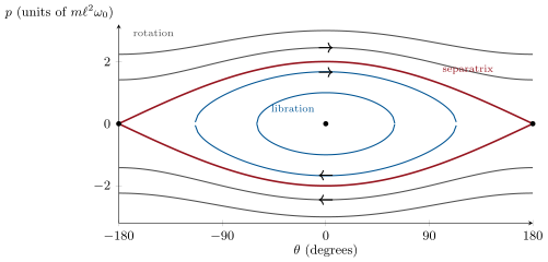
Photograph a pendulum a thousand times and plot, for each shot, its angle against its angular momentum: the points fall on a closed curve, and every possible motion of the pendulum is one such curve — small swings on nested ovals, full turns on wavy lines above and below, and between them a single crossed curve separating the two regimes. This picture, the phase portrait, is the heart of the reformulation Hamilton gave to mechanics in 1833: the state of a system is a point in the space of coordinates and momenta, its evolution is a flow in that space, and the flow is generated by a single function, the energy, through two beautifully symmetric first-order equations. The reward is not easier calculations — Lagrange usually wins there — but the right geometry: the flow conserves phase-space volume, which will found statistical physics; and its algebraic skeleton, the Poisson bracket, is precisely what quantum mechanics will promote into the commutator. This chapter is the hinge between the mechanics of things and the physics of the twentieth century.

2.1 From Lagrange to Hamilton

Definition 2.1 (Hamiltonian and canonical equations)

For a system with Lagrangian $L(q, \dot q, t)$ , express the velocities in terms of the momenta $p_i = \partial L/\partial\dot q_i$ and define the Hamiltonian as the Legendre transform

H(q, p, t) = \sum_i p_i\dot q_i - L ,

a function of the coordinates and the momenta. The $2n$ -dimensional space of the $(q_1, \dots, q_n, p_1, \dots, p_n)$ is the phase space; one point of it — one state — determines the entire future and past of the system through the canonical equations of Theorem 2.2.

Theorem 2.2 (Hamilton’s equations)

The Euler–Lagrange equations are equivalent to the $2n$ first-order equations

\dot q_i = \frac{\partial H}{\partial p_i} , \qquad \dot p_i = -\frac{\partial H}{\partial q_i} .

Proof. Differentiate $H = \sum p_i\dot q_i - L$ as a function of $(q, p, t)$ : $\dd H = \sum(\dot q_i\,\dd p_i + p_i\,\dd\dot q_i) - \sum( \partial_{q_i}L\,\dd q_i + \partial_{\dot q_i}L\,\dd\dot q_i) - \partial_tL\,\dd t$ . The $\dd\dot q_i$ terms cancel by the definition of $p_i$ — the whole point of the Legendre transform — leaving $\dd H = \sum(\dot q_i\,\dd p_i - \partial_{q_i}L\,\dd q_i) - \partial_tL\,\dd t$ . Reading off the partial derivatives: $\partial H/\partial p_i = \dot q_i$ and $\partial H/\partial q_i = -\partial L/\partial q_i$ , which by Euler–Lagrange is $-\dot p_i$ . (Also $\partial_tH = -\partial_tL$ .) ∎

Proposition 2.3 (What $H$ is)

$H$ coincides with the energy function $h$ of the previous chapter: along a motion, $\dd H/\dd t = \partial H/\partial t$ , so $H$ is conserved whenever it has no explicit time dependence; and when the kinetic energy is quadratic in the velocities with time-independent constraints, $H = E_k + E_p$ , the mechanical energy — now written in the variables $(q, p)$ .

Proof. $\dd H/\dd t = \sum(\partial_{q_i}H\,\dot q_i + \partial_{p_i}H\,\dot p_i) + \partial_tH = \sum(\partial_{q_i}H\,\partial_{p_i}H - \partial_{p_i}H\,\partial_{q_i}H) + \partial_tH = \partial_tH$ : the symmetry of the canonical equations makes the sum cancel identically. The identification with $E_k + E_p$ is Proposition 1.14. ∎

Example 2.4 (Two Hamiltonians)

Mass on a spring: $p = m\dot x$ , so

H = \frac{p^2}{2m} + \frac12 kx^2 ;

the canonical equations $\dot x = p/m$ , $\dot p = -kx$ are the familiar pair. Pendulum: $p = m\ell^2\dot\theta$ and

H = \frac{p^2}{2m\ell^2} - mg\ell\cos\theta .

In both cases $H$ is the energy, constant on each motion: the motions are the level curves of $H$ in the $(q,p)$ plane.

Method 2.5 (The Hamiltonian recipe)

(1) From $L$ , compute the momenta $p_i = \partial L/\partial\dot q_i$ and invert for the $\dot q_i$ . (2) $H = \sum p_i\dot q_i - L$ , expressed in $(q, p)$ only — for a natural system, simply $E_k + E_p$ with $E_k$ rewritten in the momenta. (3) Write the canonical equations. (4) Draw the level curves of $H$ : for one degree of freedom they are the trajectories, and the whole qualitative motion — oscillations, rotations, equilibria, separatrices — is read off without solving anything.

2.2 Phase space

Definition 2.6 (Phase portrait, fixed points, separatrix)

The phase portrait of a system is the family of its trajectories in phase space. A fixed point is a state where both canonical equations vanish — an equilibrium: a minimum of the potential appears as a centre surrounded by closed curves, a maximum as a saddle through which passes a separatrix, the trajectory that divides phase space into regions of qualitatively different motion.

Example 2.7 (The pendulum’s phase portrait)

For $H = p^2/2m\ell^2 - mg\ell\cos\theta$ : closed ovals around $(0, 0)$ — librations, the ordinary swings; wavy curves at $|p|$ large — rotations, the pendulum turning over the top; and through the saddles at $\theta = \pm\pi$ the separatrix, of energy $E = +mg\ell$ , on which the pendulum takes an infinite time to reach the top. A state on the separatrix is the swing launched exactly hard enough to arrive at the inverted position with nothing to spare.

The pendulum’s phase portrait: level curves of H. Closed ovals (swings) circulate clockwise around the centre; above and below the separatrix, the pendulum rotates. The saddles at ± 180 are the inverted equilibrium. — The pendulum’s phase portrait: level curves of $H$ . Closed ovals (swings) circulate clockwise around the centre; above and below the separatrix, the pendulum rotates. The saddles at $\pm 180^\circ$ are the inverted equilibrium.

Theorem 2.8 (Liouville’s theorem)

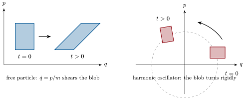
The Hamiltonian flow preserves phase-space volume: if a region of initial states is carried along by the canonical equations, its volume (its area, for one degree of freedom) never changes — whatever its shape becomes.

Proof. The flow in phase space has velocity field $(\dot q_i, \dot p_i) = (\partial_{p_i}H, -\partial_{q_i}H)$ . Its divergence is

\sum_i\Big(\frac{\partial\dot q_i}{\partial q_i} + \frac{\partial\dot p_i}{\partial p_i}\Big) = \sum_i\Big(\frac{\partial^2H}{\partial q_i\partial p_i} - \frac{\partial^2H}{\partial p_i\partial q_i}\Big) = 0 :

the flow is incompressible, and an incompressible flow transports volumes unchanged, as for the fluids of the Year 2 volume. (The formal step from zero divergence to conserved volume is the transport theorem proved there.) ∎

Remark 2.9 (Why Liouville matters)

Nothing in Newton’s formulation suggests that anything is incompressible. In the Hamiltonian picture it is automatic — and it is the licence for statistical physics: when we describe a gas of $10^{23}$ molecules by a cloud of points in phase space, Liouville’s theorem says the cloud flows like an incompressible fluid, so “number of states in a phase-space volume” is a quantity dynamics itself cannot create or destroy. The microcanonical postulate of statistical physics, later in this volume, stands on exactly this.

Liouville’s theorem: the flow deforms a region of initial states — shearing it, turning it — but its area is exactly conserved.

2.3 Poisson brackets

Definition 2.10 (Poisson bracket)

The Poisson bracket of two functions $f(q, p, t)$ and $g(q, p, t)$ on phase space is

\{f, g\} = \sum_i\Big( \frac{\partial f}{\partial q_i}\frac{\partial g}{\partial p_i} - \frac{\partial f}{\partial p_i}\frac{\partial g}{\partial q_i}\Big) .

It is antisymmetric, linear in each argument, obeys the product rule $\{f, gh\} = \{f, g\}h + g\{f, h\}$ , and satisfies for the coordinates themselves the canonical relations

\{q_i, p_j\} = \delta_{ij} , \qquad \{q_i, q_j\} = \{p_i, p_j\} = 0 .

Theorem 2.11 (Evolution as a bracket)

Along any motion,

\frac{\dd f}{\dd t} = \{f, H\} + \frac{\partial f}{\partial t} .

In particular a quantity without explicit time dependence is conserved if and only if its bracket with the Hamiltonian vanishes; and the canonical equations themselves are $\dot q_i = \{q_i, H\}$ , $\dot p_i = \{p_i, H\}$ : the Hamiltonian generates time evolution.

Proof. Chain rule plus the canonical equations: $\dd f/\dd t = \sum( \partial_{q_i}f\,\dot q_i + \partial_{p_i}f\,\dot p_i) + \partial_tf = \sum(\partial_{q_i}f\,\partial_{p_i}H - \partial_{p_i}f\, \partial_{q_i}H) + \partial_tf$ . ∎

Example 2.12 (Brackets of angular momentum)

For one particle, $L_z = xp_y - yp_x$ and its cyclic companions. A direct computation from the canonical relations gives

\{L_x, L_y\} = L_z , \qquad \{L_y, L_z\} = L_x , \qquad \{L_z, L_x\} = L_y ,

and $\{L^2, L_z\} = 0$ : the components of angular momentum do not “commute” with each other, but each commutes with the total square. Remember the shape of these relations — they will return, verbatim, as commutators in quantum mechanics, where they dictate everything about atomic structure.

Remark 2.13 (The doorway to quantum mechanics)

Dirac observed in 1925 that the whole of quantum mechanics is obtained by keeping the algebra of Hamiltonian mechanics and replacing the Poisson bracket by the commutator of operators divided by $\iu\hbar$ : $\{q, p\} = 1$ becomes $[\hat x, \hat p] = \iu\hbar$ , conservation is still “bracket with $H$ vanishes”, and time evolution is still generated by the Hamiltonian. The classical theory carries, in its bones, the skeleton of the quantum one; the chapters on quantum mechanics will make this correspondence explicit.

2.4 Action and adiabatic invariants

Definition 2.14 (Action variable)

For a one-degree-of-freedom system oscillating on a closed phase trajectory, the action variable is the enclosed area divided by $2\pi$ :

I = \frac{1}{2\pi}\oint p\,\dd q .

Proposition 2.15 (Action of the harmonic oscillator)

For $H = p^2/2m + \tfrac12 m\omega^2q^2$ at energy $E$ , the trajectory is an ellipse of semi-axes $\sqrt{2E/m\omega^2}$ and $\sqrt{2mE}$ , enclosing the area $2\pi E/\omega$ : hence

I = \frac{E}{\omega} , \qquad E = \omega I ,

and the oscillation frequency is $\partial E/\partial I = \omega$ , as it should be.

Proof. Area of an ellipse, $\pi ab = \pi\sqrt{2E/m\omega^2}\sqrt{2mE} = 2\pi E/\omega$ . ∎

Proposition 2.16 (Adiabatic invariance)

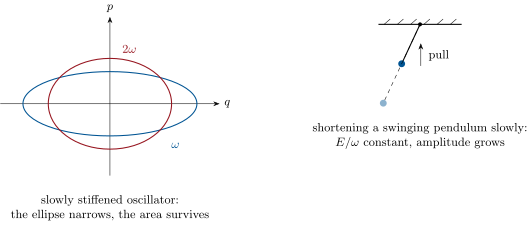
If a parameter of the system (a length, a stiffness, a field) is varied slowly — over many oscillation periods — the energy changes, the frequency changes, but the action $I$ stays constant to an excellent approximation: $I$ is an adiabatic invariant. For the slowly modified oscillator, $E/\omega$ is thus conserved: stiffen the spring slowly to double $\omega$ and the energy doubles with it.

Partial proof. For the oscillator with slowly varying $\omega(t)$ : over one period the work done by the changing parameter can be computed by averaging; the calculation (guided in Exercise 2.11) gives $\dot E/E = \dot\omega/\omega$ , i.e. $\dd(E/\omega)/\dd t = 0$ at leading order. The general statement, for any slowly deformed oscillating system, is admitted — it is the reason planetary orbits survive slow perturbations, and the starting point of the “old quantum theory” below. ∎

Adiabatic invariance. Left: as is slowly doubled, the phase ellipse changes shape at constant area, so E = I doubles. Right: hoisting the string of a swinging pendulum feeds energy into the swing in just the proportion that keeps I = E/ fixed. — Adiabatic invariance. Left: as $\omega$ is slowly doubled, the phase ellipse changes shape at constant area, so $E = \omega I$ doubles. Right: hoisting the string of a swinging pendulum feeds energy into the swing in just the proportion that keeps $I = E/\omega$ fixed.

Remark 2.17 (The old quantum theory)

Why do atoms have discrete energies? The first quantitative answer (Bohr 1913, Sommerfeld 1915) was written in the language of this chapter: among all classical motions, nature keeps those whose action integral is a whole number of Planck’s constants,

\oint p\,\dd q = nh .

Applied to the harmonic oscillator this gives $E_n = n\hbar\omega$ (missing only the half of the true $\big(n + \tfrac12\big)\hbar \omega$ ); applied to a particle in a box it gives exactly the levels of the Year 2 volume; applied to the hydrogen atom (Problem 2.1) it gives the measured spectrum to four figures. The rule was quantitatively right and conceptually provisional — and because action is an adiabatic invariant, the quantum number $n$ does not change under slow perturbations, which is why such a rule could work at all. The true theory begins five chapters from here.

A strobed pendulum: positions crowd near the turning points, where the bob lingers, and spread at the bottom, where it hurries — a photograph of the phase-space portrait this chapter draws with equations.

2.5 Exercises

Exercise 2.1 ★

For the mass on a spring: (a) construct $H$ from $L$ and check $H = E_k + E_p$ ; (b) write the canonical equations and verify they reproduce $\ddot x = -\omega^2x$ ; (c) show the trajectories are ellipses in the $(x, p)$ plane and give their semi-axes at energy $E$ ; (d) in what sense does the representative point move clockwise?

Solution

Solution of Exercise 2.1.

(a) $p = m\dot x$ , $H = p\dot x - L = p^2/2m + \tfrac12 kx^2 = E_k + E_p$ . (b) $\dot x = p/m$ , $\dot p = -kx$ , hence $\ddot x = -(k/m)x$ . (c) $H = E$ is the ellipse $x^2/(2E/k) + p^2/(2mE) = 1$ : semi-axes $\sqrt{2E/k}$ and $\sqrt{2mE}$ . (d) At the rightmost point ( $x > 0$ , $p = 0$ ), $\dot p = -kx < 0$ : the point moves downward — clockwise, always.

Exercise 2.2 ★

The bead on the rotating hoop of the previous chapter has $L = \tfrac12 mR^2\dot\theta^2 + \tfrac12 m\omega^2R^2\sin^2\theta + mgR\cos\theta$ . (a) Compute $p$ and $H$ . (b) Is $H$ conserved? Is it the mechanical energy? (c) Sketch the level curves of $H$ for $\omega^2 < g/R$ and $\omega^2 > g/R$ , using the effective potential of that chapter. (d) Identify the centres, the saddles and the separatrices in the fast case.

Solution

Solution of Exercise 2.2.

(a) $p = mR^2\dot\theta$ ; $H = p^2/2mR^2 - \tfrac12 m\omega^2R^2 \sin^2\theta - mgR\cos\theta = p^2/2mR^2 + U_{\text{eff}}(\theta)$ . (b) Conserved ( $H$ has no explicit $t$ ), but it is $h$ , not the mechanical energy: the motor’s work is missing from it. (c) The level curves are $p = \pm\sqrt{2mR^2(H - U_{\text{eff}})}$ : for slow rotation, ovals around $(0, 0)$ and a separatrix through the saddle at $\theta = \pi$ ; for fast rotation, two families of ovals around $(\pm\theta_{\text{eq}}, 0)$ . (d) Fast case: centres at $\pm\theta_{\text{eq}}$ ; saddles at $\theta = 0$ and $\theta = \pi$ ; through $\theta = 0$ passes a figure-of-eight separatrix enclosing the two centres (small oscillations hop the bottom), and through $\pi$ the outer separatrix beyond which the bead circulates over the top.

Exercise 2.3 ★

A ball bounces elastically on the floor, $H = p^2/2m + mgz$ ( $z > 0$ ). (a) Draw the phase trajectory for one flight and the whole bouncing motion. (b) What does the elastic bounce do to the representative point? (c) Compute the enclosed area for maximum height $z_{\max}$ , and the action $I$ . (d) The Bohr–Sommerfeld rule $\oint p\,\dd z = nh$ applied to a bouncing neutron ( $m = 1.67 \times 10^{-27}\,\mathrm{kg}$ ) gives quantized bounce heights: estimate the lowest, and compare with the $15\,\text{µ}\mathrm{m}$ measured in the gravitational quantum-states experiment of 2002.

Solution

Solution of Exercise 2.3.

(a) One flight is the arc $p = \pm\sqrt{2m^2g(z_{\max} - z)}$ — a parabola lying on its side, traversed from $(0, +p_0)$ up to $(z_{\max}, 0)$ and back down to $(0, -p_0)$ . (b) The bounce maps $(0, -p_0)$ to $(0, +p_0)$ : a vertical segment closing the loop. (c) $\oint p\,\dd z = 2\int_0^{z_{\max}}m\sqrt{2g(z_{\max} - z)}\,\dd z = \tfrac43 m\sqrt{2g}\,z_{\max}^{3/2}$ , and $I$ is that over $2\pi$ . (d) $z_n = \big[3nh/(4m\sqrt{2g})\big]^{2/3}$ : for a neutron, $z_1 = (6.7 \times 10^{-8})^{2/3} = 17\,\text{µ}\mathrm{m}$ — the right order: the Grenoble experiment found the lowest gravitational quantum state near $15\,\text{µ}\mathrm{m}$ (the exact treatment, with the true wave functions, gives $14\,\text{µ}\mathrm{m}$ ).

Exercise 2.4 ★

From the canonical relations alone, compute (a) $\{x^2, p\}$ ; (b) $\{xp, H\}$ for $H = p^2/2m + E_p(x)$ , and interpret the two terms (this bracket drives the virial theorem); (c) $\{L_z, x\}$ and $\{L_z, p_x\}$ ; (d) show that if $\{f, H\} = 0$ and $\{g, H\} = 0$ then $\{f, g\}$ is also conserved (use the Jacobi identity, admitted: $\{f,\{g,h\}\} + \{g,\{h,f\}\} + \{h,\{f,g\}\} = 0$ ).

Solution

Solution of Exercise 2.4.

(a) $\{x^2, p\} = 2x$ . (b) $\{xp, H\} = p^2/m - x\,E_p'(x) = 2E_k - x\,E_p'$ : on a bound motion the time average of $\dd(xp)/\dd t$ vanishes, so $\langle 2E_k\rangle = \langle x\,E_p'\rangle$ — the virial theorem (for $E_p \propto x^2$ : $\langle E_k\rangle = \langle E_p\rangle$ ; for $\propto -1/r$ : $2\langle E_k\rangle = -\langle E_p\rangle$ ). (c) $\{L_z, x\} = y$ , $\{L_z, p_x\} = p_y$ : $L_z$ generates rotations of both positions and momenta. (d) Jacobi with $h = H$ : $\{\{f, g\}, H\} = -\{\{g, H\}, f\} - \{\{H, f\}, g\} = 0$ .

Exercise 2.5 ★★

The pendulum near its separatrix. (a) Give the separatrix energy and the maximum $|p|$ on it. (b) Show that on the separatrix $p = \pm 2m\ell^2\omega_0\cos(\theta/2)$ with $\omega_0 = \sqrt{g/\ell}$ . (c) Using $\dot\theta = p/m\ell^2$ , show the time to go from $\theta$ to the top diverges logarithmically. (d) A real pendulum released just below the separatrix hangs near the inverted position for a long moment before swinging back — relate this to (c), and to the slowing down seen near every saddle.

Solution

Solution of Exercise 2.5.

(a) $E_{\text{sep}} = mg\ell$ (the energy of the inverted rest position); maximum $|p| = 2m\ell^2\omega_0$ at the bottom. (b) From $p^2/2m\ell^2 = mg\ell(1 + \cos\theta) = 2mg\ell\cos^2(\theta/2)$ . (c) $\dot\theta = 2\omega_0\cos(\theta/2)$ separates: $\omega_0t = \ln\tan(\theta/4 + \pi/4)$ , which diverges as $\theta \to \pi$ : the top is approached but never reached. (d) Just below the separatrix the motion shadows it: the pendulum creeps into the neighbourhood of the saddle, lingers — the logarithm — and finally falls back; every saddle point slows trajectories logarithmically, which is why a stick balanced not quite perfectly seems to hesitate before falling.

Exercise 2.6 ★★

A charged particle in a magnetic field has $H = (\vect p - q\vect A)^2/2m$ with $\vect p$ the canonical momentum of the previous chapter. (a) Write the canonical equations for $\vect A = \tfrac12 B(-y, x, 0)$ and check they give the cyclotron motion. (b) Show $H = \tfrac12 m\vect v^{\,2}$ : the magnetic field does no work. (c) Compute the bracket of the two conserved quantities $\pi_x = p_x - \tfrac12 qBy$ and $\pi_y = p_y + \tfrac12 qBx$ (check first that each is conserved), and show $\{\pi_x, \pi_y\} = -qB$ : two conserved quantities whose bracket is a constant. (d) Use Exercise 2.4(d) to explain why no third independent conserved quantity was to be expected from them.

Solution

Solution of Exercise 2.6.

(a) $\dot{\vect r} = (\vect p - q\vect A)/m$ and $\dot p_x = -\partial H/\partial x = (q/m)(\vect p - q\vect A)\cdot\partial_x\vect A$ , etc.; eliminating $\vect p$ reproduces $m\ddot x = qB\dot y$ , $m\ddot y = -qB\dot x$ . (b) $H = (\vect p - q\vect A)^2/2m = \tfrac12 m\vect v^{\,2}$ : kinetic energy only — constant, since the magnetic force is perpendicular to $\vect v$ . (c) With $m\dot x = p_x + \tfrac12 qBy$ : $\pi_x = p_x - \tfrac12 qBy = m\dot x - qBy$ , whose conservation is the first equation of motion (similarly $\pi_y$ ); in the bracket only two terms survive: $\{p_x, \tfrac12 qBx\} = -\tfrac12 qB$ and $\{-\tfrac12 qBy, p_y\} = -\tfrac12 qB$ , total $-qB$ . ( $\pi_x/qB$ and $\pi_y/qB$ are, up to signs, the coordinates of the guiding centre of the circle.) (d) By Exercise 2.4(d) the bracket of two conserved quantities is conserved — here it is the constant $-qB$ , which is conserved trivially and teaches nothing new: no third quantity appears.

Exercise 2.7 ★★

Liouville, by hand. (a) For the free particle, the flow is $q \to q + pt/m$ , $p \to p$ : show a rectangle becomes a parallelogram of the same area. (b) For the harmonic oscillator, show the flow is a rotation (in suitable units) and conclude. (c) For the damped oscillator $\ddot x = -\omega^2x - \gamma\dot x$ , write the flow’s divergence in the $(x, v)$ plane and show areas shrink as $\eu^{-\gamma t}$ : damping is not Hamiltonian. (d) Where does the lost area “go” physically?

Solution

Solution of Exercise 2.7.

(a) The map $(q, p) \mapsto (q + pt/m, p)$ is a shear: base and height of the rectangle are unchanged, area too (determinant $1$ ). (b) In variables $(x\sqrt{m\omega}, p/\sqrt{m\omega})$ the flow is a rigid rotation at rate $\omega$ ; rotations preserve area, and the change of variables has determinant $1$ . (c) The velocity field $(v, -\omega^2x - \gamma v)$ has divergence $-\gamma$ : any area contracts as $\eu^{-\gamma t}$ , spiralling onto the origin — impossible for a Hamiltonian flow. (d) Into the ignored degrees of freedom: the air molecules and the wire’s phonons, whose phase-space volume grows by at least as much — the seed of the second law.

Exercise 2.8 ★★

Planar motion in a central potential, $H = (p_r^2 + p_\varphi^2/r^2)/2m + E_p(r)$ . (a) Write the four canonical equations. (b) Show $\{ p_\varphi, H\} = 0$ and identify the conservation law. (c) Reduce to a one-dimensional radial Hamiltonian with an effective potential. (d) For $E_p = -k/r$ , locate the circular orbit at given $p_\varphi$ and give its energy — to be quantized in Problem 2.1.

Solution

Solution of Exercise 2.8.

(a) $\dot r = p_r/m$ , $\dot\varphi = p_\varphi/mr^2$ , $\dot p_r = p_\varphi^2/mr^3 - E_p'(r)$ , $\dot p_\varphi = 0$ . (b) $H$ does not contain $\varphi$ : $\{p_\varphi, H\} = -\partial H/\partial\varphi = 0$ ; conservation of angular momentum. (c) $H_{\text{rad}} = p_r^2/2m + U_{\text{eff}}(r)$ with $U_{\text{eff}} = p_\varphi^2/2mr^2 + E_p(r)$ . (d) $U_{\text{eff}}' = 0$ : $r_{\text{c}} = p_\varphi^2/mk$ , and $E = U_{\text{eff}}(r_{\text{c}}) = -mk^2/2p_\varphi^2$ .

Exercise 2.9 ★★

(a) Verify $\{L_x, L_y\} = L_z$ from the canonical relations. (b) Deduce the other two brackets by cyclic permutation. (c) Show $\{L^2, L_z\} = 0$ . (d) A rigid body rotates freely: taking $H = L^2/2J$ (sphere-symmetric inertia), show all three $L_i$ are conserved; what about a body with unequal moments of inertia (answer qualitatively from the brackets)?

Solution

Solution of Exercise 2.9.

(a) $\{L_x, L_y\} = \{yp_z - zp_y,\ zp_x - xp_z\}$ : the only non-vanishing canonical brackets give $yp_x\{p_z, z\} + xp_y\{z, p_z\} = -yp_x + xp_y = L_z$ . (b) Cyclic relabelling $x \to y \to z \to x$ gives the other two. (c) $\{L^2, L_z\} = 2L_x\{L_x, L_z\} + 2L_y\{L_y, L_z\} = -2L_xL_y + 2L_yL_x = 0$ . (d) For $H = L^2/2J$ , each $\{L_i, H\} = 0$ : $\vect L$ fixed. With $H = \sum L_i^2/2J_i$ and unequal $J_i$ : $\{L_x, H\} = L_yL_z(1/J_y - 1/J_z) \neq 0$ — only $L^2$ and $H$ survive, and the body tumbles (the tennis-racket theorem of the Year 2 volume’s rigid-body chapter lives here).

Exercise 2.10 ★★★

Old-quantum levels. (a) Show that $\oint p\,\dd q = nh$ applied to the harmonic oscillator gives $E_n = n\hbar\omega$ , using Proposition 2.15. (b) Apply it to the particle in a box of length $a$ and recover exactly $E_n = n^2h^2/8ma^2$ . (c) For a diatomic molecule modelled as an oscillator of stiffness $k = 1.9 \times 10^{3}\,\mathrm{N}/\mathrm{m}$ and reduced mass $1.14 \times 10^{-26}\,\mathrm{kg}$ (carbon monoxide), compute $\hbar\omega$ in eV and the wavelength of the $n = 1 \to 0$ emission; in which spectral range does it fall? (d) The true levels are $(n + \tfrac12)\hbar\omega$ : does the missing half change the emitted wavelengths? What experiment does detect the zero-point half?

Solution

Solution of Exercise 2.10.

(a) $\oint p\,\dd q = 2\pi I = 2\pi E/\omega = nh$ gives $E_n = n\hbar\omega$ . (b) Back and forth at constant $|p|$ : $2pa = nh$ , $p = nh/2a$ , $E = p^2/2m = n^2h^2/8ma^2$ — exactly the infinite well of the Year 2 volume. (c) $\omega = \sqrt{k/\mu} = 4.1 \times 10^{14}\,\mathrm{rad}/\mathrm{s}$ , $\hbar\omega = 4.3 \times 10^{-20}\,\mathrm{J} = 0.27\,\mathrm{eV}$ , $\lambda = hc/ \hbar\omega = 4.6\,\text{µ}\mathrm{m}$ : mid-infrared (the CO fundamental band, used to trace the gas in space). (d) No: differences of levels are unchanged by the common half. The zero-point energy shows in comparisons that depend on the absolute level — isotope shifts of dissociation energies (H $_2$ versus D $_2$ ), or vibrations that persist at absolute zero in crystals.

Exercise 2.11 ★★★

Adiabatic invariance of $E/\omega$ , derived. A mass on a spring whose stiffness $k(t)$ grows slowly. (a) Show $\dot E = \tfrac12\dot k\, x^2$ along the exact motion. (b) Average over one period at fixed $k$ : using $\langle\tfrac12 kx^2\rangle = E/2$ , show $\langle\dot E\rangle = \dot k\,E/2k$ . (c) Conclude $\dd\ln E = \tfrac12\dd\ln k = \dd\ln \omega$ , hence $E/\omega$ constant. (d) A pendulum swinging with amplitude $\theta_0 = 5^\circ$ has its string slowly shortened from $1.0\,\mathrm{m}$ to $0.5\,\mathrm{m}$ : find the new amplitude and the factor by which its energy grew, and say where the energy came from.

Solution

Solution of Exercise 2.11.

(a) $E = p^2/2m + \tfrac12 k(t)x^2$ , so along a motion $\dot E = \partial E/\partial t = \tfrac12\dot kx^2$ . (b) Over one period at essentially fixed $k$ , $\langle\tfrac12 kx^2\rangle = E/2$ , so $\langle\dot E\rangle = \dot k\,E/2k$ . (c) $\dd\ln E = \tfrac12\dd\ln k$ ; since $\omega = \sqrt{k/m}$ , $\dd\ln\omega = \tfrac12\dd\ln k$ too: $E/\omega$ is invariant. (d) $\omega \propto \ell^{-1/2}$ grows by $\sqrt2$ , so $E$ grows by $\sqrt2 \approx 1.41$ . With $E = \tfrac12 mg\ell\theta_0^2$ , $\theta_0 \propto \ell^{-3/4}$ : $\theta_0' = 5^\circ \times 2^{3/4} = 8.4^\circ$ . The energy is supplied by whoever pulls the string: the tension exceeds $mg\cos\theta$ on average (centrifugal term), so hoisting does net positive work on the swing.

Exercise 2.12 ★★★

The area inside the pendulum’s separatrix is a number of quantum states. (a) Show $\oint p\,\dd\theta$ around the separatrix equals $16m\ell^2\omega_0$ . (b) By the Bohr–Sommerfeld rule, the number of quantum states with energies below the separatrix is $N \approx 16m\ell^2\omega_0/h$ : evaluate it for a gram mass on a $10\,\mathrm{cm}$ string. (c) Evaluate it for an ammonia-like molecular oscillator: $m \sim 1 \times 10^{-26}\,\mathrm{kg}$ , $\ell \sim 1 \times 10^{-10}\,\mathrm{m}$ , $\omega_0 \sim 1 \times 10^{14}\,\mathrm{rad}/\mathrm{s}$ . (d) Conclude: where is the border between mechanics that needs $\hbar$ and mechanics that does not?

Solution

Solution of Exercise 2.12.

(a) $\oint p\,\dd\theta = 2\int_{-\pi}^{\pi}2m\ell^2\omega_0 \cos(\theta/2)\,\dd\theta = 4m\ell^2\omega_0\big[2\sin(\theta/2) \big]_{-\pi}^{\pi} = 16m\ell^2\omega_0$ . (b) $\omega_0 = 9.9\,\mathrm{rad}/\mathrm{s}$ : $16 \times 10^{-3} \times 10^{-2} \times 9.9 = 1.6 \times 10^{-3}\,\mathrm{J}\,\mathrm{s}$ , i.e. $N \approx 2.4 \times 10^{30}$ states: the quantum graininess of a laboratory pendulum is thirty orders of magnitude below anything observable. (c) $16 \times 10^{-26} \times 10^{-20} \times 10^{14} = 1.6 \times 10^{-31}\,\mathrm{J}\,\mathrm{s}$ , i.e. $N \approx 240$ : a molecular libration holds only a few hundred quantum states, and its low levels are individually resolved by spectroscopy. (d) The border is where the phase-space areas of the motion are a modest multiple of $h$ : molecules and below are quantum; anything visible is classical.

2.6 Problem: The old quantum theory and the hydrogen atom

Problem 2.1

Weekend problem — quantizing phase space, weighing the Rydberg

In 1913 Bohr computed the spectrum of hydrogen from planetary mechanics plus one quantum rule; Sommerfeld recognised the rule as a statement about phase-space area. This problem rebuilds their calculation with this chapter’s tools. Data: $m_{\text{e}} = 9.11 \times 10^{-31}\,\mathrm{kg}$ , $e = 1.60 \times 10^{-19}\,\mathrm{C}$ , $1/4\pi\varepsilon_0 = 8.99 \times 10^{9}\,\mathrm{N}\,\mathrm{m}^{2}/\mathrm{C}^{2}$ , $h = 6.63 \times 10^{-34}\,\mathrm{J}\,\mathrm{s}$ , $c = 3.00 \times 10^{8}\,\mathrm{m}/\mathrm{s}$ . Write $k = e^2/4\pi\varepsilon_0$ .

Part I — The Kepler Hamiltonian. An electron moves in the plane around a fixed proton.

Justify treating the proton as fixed (mass ratio), and write the Hamiltonian $H = \dfrac{p_r^2}{2m_{\text{e}}} + \dfrac{p_\varphi^2}{2m_{\text{e}}r^2} - \dfrac{k}{r}$ .
Write the four canonical equations.
Show $p_\varphi$ is conserved and name it.
Reduce the radial motion to the effective potential $U_{\text{eff}}(r) = p_\varphi^2/2m_{\text{e}}r^2 - k/r$ and sketch it.
Locate the circular orbit: $r_{\text{c}} = p_\varphi^2/m_{\text{e}}k$ .
Show its energy is $E = -k/2r_{\text{c}} = -m_{\text{e}}k^2/2p_\varphi^2$ , and check that it is half the potential energy (the virial ratio of the Year 1 volume’s gravitational orbits).

Part II — The classical orbit.

For a circular orbit of radius $r$ , find the speed $v$ and the orbital frequency $f_{\text{orb}}$ as functions of $r$ .
An orbit of atomic size, $r = 0.05\,\mathrm{nm}$ : compute $v$ (and $v/c$ ), $f_{\text{orb}}$ , and the energy in eV.
Compute the angular momentum $p_\varphi$ of that orbit and compare it with $\hbar = h/2\pi$ : what does the closeness suggest?
Classically, an orbiting electron is an oscillating dipole and radiates (Year 2 volume) at $f_{\text{orb}}$ ; its energy decays in about $1 \times 10^{-11}\,\mathrm{s}$ . State the two fatal predictions this makes for atoms, and what is observed instead.
Which feature of the observed spectra (discrete lines, combination rule $1/\lambda = R_H(1/n^2 - 1/n'^2)$ ) suggested discrete energy levels?
Explain why an adiabatic invariant is the natural candidate for a quantity that takes fixed universal values (recall Proposition 2.16).

Part III — Quantization. Impose Sommerfeld’s rule on the angular motion of the circular orbit: $\oint p_\varphi\,\dd\varphi = nh$ , $n = 1, 2, 3, \dots$

Show the rule reads $p_\varphi = n\hbar$ .
Deduce the allowed radii $r_n = n^2a_0$ with $a_0 = \hbar^2/m_{\text{e}}k$ , and compute $a_0$ .
Deduce the allowed energies $E_n = -E_{\text{I}}/n^2$ with $E_{\text{I}} = m_{\text{e}}k^2/2\hbar^2$ , and compute $E_{\text{I}}$ in joules and eV.
Compute the speed on the first orbit and check $v_1/c = k/\hbar c \approx 1/137$ (the fine-structure constant).
A photon carries the energy of a transition: derive the Rydberg formula and the value of $R_H = E_{\text{I}}/hc$ ; compare with the measured $1.097 \times 10^{7}\,\mathrm{m}^{-1}$ .
Compute the wavelengths of the transitions $2 \to 1$ , $3 \to 2$ and $\infty \to 2$ ; which one is visible, and what colour?
The ionised helium ion He $^+$ is hydrogen with nuclear charge $2e$ : how do $a_0$ and $E_{\text{I}}$ scale, and where does its $2 \to 1$ line fall?

Part IV — Confrontation.

Compute the orbital frequency $f_{\text{orb}}(n)$ and the transition frequency $\nu_{n \to n-1}$ for $n = 2$ , $10$ , $100$ , and show their ratio tends to $1$ as $n$ grows.
This is Bohr’s correspondence principle: state it in one sentence.
The rule $p_\varphi = n\hbar$ starts at $n = 1$ : what absurdity would $n = 0$ mean for a circular orbit?
Quantum mechanics will keep $E_n = -E_{\text{I}}/n^2$ exactly, yet discard the orbits: name two measurable facts the orbit picture gets wrong (size of the ground state’s angular momentum; existence of states with the same $n$ and different shapes).
The muon is an electron $207$ times heavier: for muonic hydrogen, compute $a_0^\mu$ and $E_{\text{I}}^\mu$ , and explain why muonic atoms probe the nucleus.
Summarise the named result: one adiabatic invariant, set equal to whole numbers of $h$ , yields $a_0 = 52.9\,\mathrm{pm}$ , $E_{\text{I}} = 13.6\,\mathrm{eV}$ and the hydrogen spectrum to four figures — and hands the true theory its two central constants.

Solution

Solution of Problem 2.1.

1. $m_{\text{p}}/m_{\text{e}} = 1836$ : the proton moves 1836 times less; $H$ as stated, in the plane of the orbit. 2. $\dot r = p_r/m_{\text{e}}$ , $\dot\varphi = p_\varphi/m_{\text{e}}r^2$ , $\dot p_r = p_\varphi^2/m_{\text{e}}r^3 - k/r^2$ , $\dot p_\varphi = 0$ . 3. $\varphi$ absent from $H$ : $p_\varphi$ , the angular momentum, is conserved. 4. $U_{\text{eff}} = p_\varphi^2/2m_{\text{e}}r^2 - k/r$ : repulsive wall at small $r$ , Coulomb tail at large $r$ , one minimum between. 5. $U_{\text{eff}}' = 0$ at $r_{\text{c}} = p_\varphi^2/m_{\text{e}}k$ . 6. $E = k/2r_{\text{c}} - k/r_{\text{c}} = -k/2r_{\text{c}} = -m_{\text{e}}k^2/2p_\varphi^2$ ; $E_p = -k/r_{\text{c}} = 2E$ : the virial ratio of any circular $1/r$ orbit. 7. $m_{\text{e}}v^2/r = k/r^2$ : $v = \sqrt{k/m_{\text{e}}r}$ , $f_{\text{orb}} = v/2\pi r = (1/2\pi)\sqrt{k/m_{\text{e}}r^3}$ . 8. $k = 2.30 \times 10^{-28}\,\mathrm{J}\,\mathrm{m}$ : $v = 2.2 \times 10^{6}\,\mathrm{m}/\mathrm{s}$ ( $v/c = 0.0075$ ), $f_{\text{orb}} = 7.2 \times 10^{15}\,\mathrm{Hz}$ , $E = -k/2r = -2.3 \times 10^{-18}\,\mathrm{J} = -14\,\mathrm{eV}$ . 9. $p_\varphi = m_{\text{e}}vr = 1.0 \times 10^{-34}\,\mathrm{J}\,\mathrm{s} \approx \hbar$ : an atomic orbit carries an angular momentum of order $\hbar$ — Planck’s constant is built into atomic sizes. 10. Every atom should collapse in $\sim10^{-11}\,\mathrm{s}$ , its light sweeping continuously to shorter wavelengths. Observed: atoms are eternal and emit sharp, fixed lines. 11. $1/\lambda = R_H(1/n^2 - 1/n'^2)$ writes every observed frequency as a difference of terms: energy is exchanged between fixed levels $-hcR_H/n^2$ . 12. A quantity locked to universal values must not drift when the atom is gently perturbed (fields, collisions, slow changes); an adiabatic invariant is precisely what stays fixed under slow perturbation — so quantize the action. 13. $p_\varphi$ is constant on the orbit: $\oint p_\varphi\,\dd\varphi = 2\pi p_\varphi = nh$ , i.e. $p_\varphi = n\hbar$ . 14. $r_n = (n\hbar)^2/m_{\text{e}}k = n^2a_0$ , $a_0 = \hbar^2/m_{\text{e}}k = 5.29 \times 10^{-11}\,\mathrm{m} = 52.9\,\mathrm{pm}$ . 15. $E_n = -m_{\text{e}}k^2/2n^2\hbar^2 = -E_{\text{I}}/n^2$ , $E_{\text{I}} = m_{\text{e}}k^2/2\hbar^2 = 2.18 \times 10^{-18}\,\mathrm{J} = 13.6\,\mathrm{eV}$ . 16. $v_1 = k/\hbar = 2.19 \times 10^{6}\,\mathrm{m}/\mathrm{s}$ ; $v_1/c = k/\hbar c = 1/137$ : the fine-structure constant $\alpha$ , measuring how non-relativistic the atom is. 17. $h\nu = E_{n'} - E_n$ gives $1/\lambda = (E_{\text{I}}/hc)(1/n^2 - 1/n'^2)$ : $R_H = E_{\text{I}}/hc = 1.10 \times 10^{7}\,\mathrm{m}^{-1}$ , matching the measured $1.097 \times 10^{7}\,\mathrm{m}^{-1}$ to the accuracy of our constants. 18. $2 \to 1$ : $122\,\mathrm{nm}$ (far ultraviolet, Lyman $\alpha$ ); $3 \to 2$ : $656\,\mathrm{nm}$ , the visible red line that colours emission nebulae; $\infty \to 2$ : $365\,\mathrm{nm}$ , the near-ultraviolet edge of the Balmer series. 19. $k \to 2k$ : radii shrink by $2$ , $E_{\text{I}} \to 4 \times 13.6\,\mathrm{eV} = 54.4\,\mathrm{eV}$ ; the $2 \to 1$ line falls at $122\,\mathrm{nm}/4 \approx 30\,\mathrm{nm}$ , in the extreme ultraviolet. 20. $f_{\text{orb}}(n) = 2E_{\text{I}}/hn^3$ ; $\nu_{n \to n-1} = (E_{\text{I}}/h)(2n - 1)/n^2(n-1)^2$ . Ratio $\nu/f_{\text{orb}} = n^3(2n-1)/2n^2(n-1)^2$ : $3$ at $n = 2$ , $1.17$ at $n = 10$ , $1.015$ at $n = 100$ . 21. In the limit of large quantum numbers, quantum predictions must merge into the classical ones — here, the radiated frequency into the orbital frequency. 22. $n = 0$ means $p_\varphi = 0$ : a “circular orbit” of zero radius, the electron on the proton — no such motion exists. 23. Measured hydrogen has a ground state with zero angular momentum (not $\hbar$ ), and several distinct states sharing the same $n$ (the $s$ , $p$ , $d$ shapes of chemistry) — both impossible for a single circular orbit. 24. $a_0 \propto 1/m$ : $a_0^\mu = 256\,\mathrm{fm}$ ; $E_{\text{I}}^\mu = 207 \times 13.6\,\mathrm{eV} = 2.8\,\mathrm{keV}$ (X-rays). The muon orbits two hundred times closer — partly inside the nuclear charge for heavy elements — so its levels measure nuclear radii (and sharpened the modern puzzle of the proton’s size). 25. One adiabatic invariant set to $nh$ delivers $a_0 = 52.9\,\mathrm{pm}$ , $E_{\text{I}} = 13.6\,\mathrm{eV}$ , $R_H = 1.10 \times 10^{7}\,\mathrm{m}^{-1}$ — numbers the full quantum theory of Chapter 11 will keep unchanged, while replacing the orbits that produced them.

Terms defined in this chapter

See all 431 terms in the glossary