University Physics — Year 3 · Bachelor Year 3

13Perturbation Theory

Only a handful of quantum problems dissolve exactly: the box, the oscillator, hydrogen, the two-level system. Everything else — an atom in a field, a molecule’s stiffening bond, a level nudged by a neighbour — is one of those solvable skeletons wearing a small extra term. Perturbation theory is the art of treating the extra term as what it is: a correction, computed order by order in its smallness. Its first-order rule is a one-line average; its second-order rule explains why levels repel, why every atom is polarisable, and why van der Waals attraction is universal; its degenerate variant handles the delicate cases where near-equal levels reorganise entirely; and its time-dependent form — Fermi’s golden rule — is the equation behind every absorption line, decay rate, and scattering cross-section measured in a laboratory. As a running reward, the chapter ends by computing the colour of the sky.

13.1 Small shifts: the non-degenerate theory

Theorem 13.1 (Perturbative corrections)

Let $\hat H = \hat H_0 + \hat V$ with $\hat H_0$ solved ( $\hat H_0\ket n = E_n\ket n$ , spectrum non-degenerate) and $\hat V$ small. Then, order by order in $\hat V$ ,

E_n' = E_n + \bra n\hat V\ket n + \sum_{m \neq n}\frac{|\bra m\hat V\ket n|^2}{E_n - E_m} + \cdots

and the state acquires admixtures $\ket{n'} = \ket n + \sum_{m\neq n}\dfrac{\bra m\hat V\ket n}{E_n - E_m}\,\ket m + \cdots$ First order: the shift is just the average of the perturbation in the unperturbed state. Second order: couplings to other levels push $E_n$ away from them — each $m$ above pushes down, each below pushes up — so the ground state’s second-order shift is always negative. Validity: the mixing fractions $|\bra m\hat V\ket n/(E_n - E_m)|$ must be small.

Partial proof. Expand $E' = E + \epsilon_1 + \epsilon_2 + \cdots$ and $\ket{\psi} = \ket n + \ket{\psi_1} + \cdots$ in powers of $\hat V$ , insert into $(\hat H_0 + \hat V)\ket\psi = E'\ket\psi$ , and match orders. Projecting the first-order equation on $\bra n$ gives $\epsilon_1 = \bra n\hat V\ket n$ ; projecting on $\bra m$ ( $m \neq n$ ) gives the admixture coefficients; carrying those into the second-order equation and projecting on $\bra n$ again gives $\epsilon_2$ . The sign statement for the ground state: every denominator $E_0 - E_m$ is negative while the numerators are squares. ∎

Proposition 13.2 (A perturbation with an exact answer)

An oscillator of charge $q$ in a uniform field $\mathcal E$ has $\hat V = -q\mathcal E\hat x$ . Completing the square solves it exactly: the potential is the same parabola, shifted, with all levels lowered by $q^2\mathcal E^2/2m\omega^2$ . Perturbation theory must agree — and does: first order vanishes ( $\langle\hat x\rangle_n = 0$ ), and the second-order sum, in which $\hat x$ couples $n$ only to $n \pm 1$ , gives exactly $-q^2\mathcal E^2/2m\omega^2$ for every level (Exercise 13.2). One solvable case, checked both ways, is the best calibration a method can have.

Proof. The two matrix elements and their denominators give

\frac{|\bra{n+1}\hat x\ket{n}|^2}{-\hbar\omega} + \frac{|\bra{n-1}\hat x\ket n|^2}{+\hbar\omega} = \frac{\hbar}{2m\omega}\,\frac{-(n+1) + n}{\hbar\omega} = -\frac{1}{2m\omega^2} ;

multiply by $q^2\mathcal E^2$ . ∎

Level repulsion: two coupled levels never cross — as the coupling (or a parameter sweeping the bare energies) varies, the exact energies ±√ 2 + v2 avoid each other. The second-order formula is the far wing of this hyperbola; the “avoided crossing” at the centre is where perturbation theory hands over to exact diagonalisation. — Level repulsion: two coupled levels never cross — as the coupling (or a parameter sweeping the bare energies) varies, the exact energies $\pm\sqrt{\Delta^2 + v^2}$ avoid each other. The second-order formula is the far wing of this hyperbola; the “avoided crossing” at the centre is where perturbation theory hands over to exact diagonalisation.

13.2 When levels are degenerate

Theorem 13.3 (Degenerate perturbation theory)

If $E_n$ is degenerate, the formula above divides by zero — the perturbation may reorganise the degenerate states completely, and the cure is to let it: diagonalise $\hat V$ restricted to the degenerate subspace. Its eigenvalues are the first-order shifts; its eigenvectors are the correct zeroth-order states, the combinations the perturbation itself selects.

Proof. Admitted at this level. ∎

Example 13.4 (The linear Stark effect)

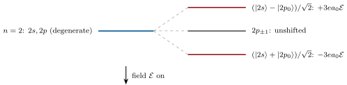
Hydrogen’s $n = 2$ level holds the degenerate $2s$ and $2p$ states. In a field $\mathcal E\vect e_z$ , $\hat V = e\mathcal E\hat z$ couples $2s$ to $2p_0$ with $\bra{2s}\hat z\ket{2p_0} = -3a_0$ : diagonalising the $2\times2$ block gives shifts

\Delta E = \pm\,3e a_0\mathcal E ,

linear in the field — while the non-degenerate ground state shifts only quadratically. At $\mathcal E = 10^{7}\,\mathrm{V}/\mathrm{m}$ : $\pm 1.6\,\mathrm{meV}$ , an easily resolved splitting. The states doing the splitting are $(\ket{2s} \mp \ket{2p_0})/\sqrt2$ — hybrids with a permanent electric dipole, possible only because degeneracy left the atom free to polarise at zeroth order. (The same $s$ – $p$ hybridisation, driven by neighbours instead of a field, is the carbon chemistry of every organic molecule.)

The linear Stark effect in hydrogen’s n = 2 shell: the field hybridises the degenerate 2s and 2p_0 into permanent-dipole states shifted by ±3ea_0 E, leaving 2p_±1 untouched at first order. — The linear Stark effect in hydrogen’s $n = 2$ shell: the field hybridises the degenerate $2s$ and $2p_0$ into permanent-dipole states shifted by $\pm3ea_0\mathcal E$ , leaving $2p_{\pm1}$ untouched at first order.

13.3 Transitions: the golden rule

Theorem 13.5 (Time-dependent perturbations)

Switch on $\hat V(t) = \hat V\cos\omega t$ at $t = 0$ . To first order, the probability of finding the system in $\ket f$ at time $t$ , having started in $\ket i$ , is

\mathcal P_{i\to f}(t) = \frac{|\bra f\hat V\ket i|^2}{4\hbar^2}\; \frac{\sin^2\!\big[(\omega_{fi} - \omega)\,t/2\big]} {\big[(\omega_{fi} - \omega)/2\big]^2} , \qquad \omega_{fi} = \frac{E_f - E_i}{\hbar} :

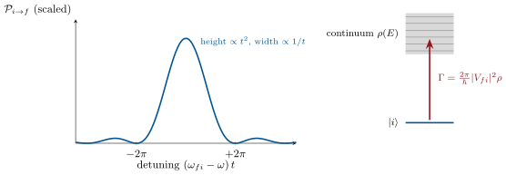
a resonance sharply peaked at $\hbar\omega = E_f - E_i$ — absorption when $E_f > E_i$ , stimulated emission for the companion term with $E_f < E_i$ . When the final states form a continuum of density $\rho(E)$ , the peak’s growth becomes a constant rate:

\Gamma_{i\to f} = \frac{2\pi}{\hbar}\, |\bra f\hat V\ket i|^2\,\rho(E_f)

— Fermi’s golden rule, the master formula of decay rates, absorption coefficients and cross-sections.

Partial proof. First-order amplitude: $c_f(t) = -\tfrac{\iu}{\hbar}\int_0^t\bra f\hat V(t')\ket i\,\eu^{\iu\omega_{fi}t'}\dd t'$ ; keeping the near-resonant exponential and integrating gives the stated $\sin^2$ form. For the continuum: as a function of the detuning $x$ , the resonance factor has height $t^2$ and width $\sim 2\pi/t$ — area $2\pi t$ — so summing over a smooth continuum replaces it by $2\pi t\,\rho$ : probability linear in $t$ , i.e. a rate. ∎

Left: the first-order transition probability against detuning — an ever-narrower, ever-taller resonance whose area grows linearly in time. Right: into a continuum, that linear growth is a constant decay rate: the golden rule.

Example 13.6 (What the golden rule runs)

Selection rules: a transition happens only if the matrix element $\bra f\hat V\ket i$ survives — for light, $\hat V \propto \hat z$ , whose parity and angular momentum kill everything except $\Delta l = \pm1$ , $\Delta m = 0, \pm1$ : the rules invoked since Chapter 10, now theorems. Rates: the hydrogen $2p$ state’s spontaneous decay computes to $1.6\,\mathrm{ns}$ (Exercise 13.8); ammonia’s maser transition, with its microwave $\omega^3$ , takes months — the $\omega^3$ in radiated rates is why radio lines (Example 12.7) live for megayears while ultraviolet lines flash in nanoseconds. Absorption spectra, photoionisation, nuclear beta decay (Chapter 25), scattering cross-sections (Chapter 15): all are this one formula with different matrix elements and state counts.

Method 13.7 (Choosing the right perturbative tool)

(1) Static question, non-degenerate level: average $\hat V$ (first order); if that vanishes by symmetry, second order — expect level repulsion. (2) Degenerate level: diagonalise $\hat V$ in the degenerate block first; the symmetry-adapted combinations do the splitting. (3) Transition rates: golden rule — one matrix element, one density of states; check selection rules before computing anything. (4) Always test the expansion: mixing fraction $|V_{mn}/(E_n - E_m)| \ll 1$ , else diagonalise exactly (two-level formula). (5) Exact solvable limits (oscillator in a field) are free calibrations: use them.

Sunset as perturbation theory: air’s molecules scatter blue light far more readily than red (the 4 of this chapter’s golden-rule kin), so the long path at the horizon strains the blue away and mails it to someone else’s noon sky. — Sunset as perturbation theory: air’s molecules scatter blue light far more readily than red (the $\omega^4$ of this chapter’s golden-rule kin), so the long path at the horizon strains the blue away and mails it to someone else’s noon sky.

13.4 Exercises

Exercise 13.1 ★

A particle in a box $[0, a]$ feels the extra potential $V(x) = \lambda x/a$ . (a) Compute the first-order shift of every level (use $\langle x\rangle = a/2$ in any box state — justify it). (b) Why is the shift the same for all levels here? (c) What is the first-order change of the spacings, and why could a measurement of transition frequencies miss this perturbation entirely? (d) When does first order stop being trustworthy?

Solution

Solution of Exercise 13.1.

(a) Every $|\varphi_n|^2$ is symmetric about $a/2$ , so $\langle x\rangle = a/2$ and $\Delta E_n = \lambda/2$ for all $n$ . (b) The symmetry, not the dynamics. (c) A common shift cancels in every difference: spectroscopy, which measures spacings, sees nothing at first order. (d) When $\lambda$ rivals the level spacings, the neglected state mixing (second order) matters.

Exercise 13.2 ★

Carry out the second-order computation of Proposition 13.2 in full: matrix elements of $\hat x$ , the two terms, the cancellation of $n$ , and the exact agreement with completing the square. Why does the state’s first-order correction not vanish although the energy’s does?

Solution

Solution of Exercise 13.2.

$\bra{n\pm1}\hat x\ket n = \sqrt{\hbar/2m\omega}\,\sqrt{n + \tfrac12 \pm \tfrac12}$ ; the two second-order terms give

\frac{q^2\mathcal E^2\hbar}{2m\omega}\Big[\frac{n+1}{-\hbar\omega} + \frac{n}{\hbar\omega}\Big] = -\frac{q^2\mathcal E^2}{2m\omega^2} ,

independent of $n$ — the exact answer. The state is corrected at first order (admixtures of $n \pm 1$ displace the wave function sideways); only the energy’s first-order piece vanishes, by parity.

Exercise 13.3 ★

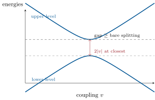
The two-level Hamiltonian $\begin{pmatrix}E_1 & v\\ v & E_2\end{pmatrix}$ , $E_1 < E_2$ , $v$ real. (a) Find the exact eigenvalues. (b) Expand for $|v| \ll E_2 - E_1$ and identify the second-order formula. (c) Show the levels repel: the gap always exceeds $E_2 - E_1$ . (d) At $E_1 = E_2$ : what does perturbation theory give, what does the exact answer give, and which theorem of the chapter reconciles them?

Solution

Solution of Exercise 13.3.

(a) $E_\pm = \bar E \pm \sqrt{(\Delta/2)^2 + v^2}$ with $\Delta = E_2 - E_1$ . (b) $E_- \approx E_1 - v^2/\Delta$ , $E_+ \approx E_2 + v^2/\Delta$ : the second-order formula, term by term. (c) The gap $2\sqrt{(\Delta/2)^2 + v^2} \ge \Delta$ , with equality only at $v = 0$ . (d) The expansion diverges; the exact answer gives $\pm|v|$ — which is precisely what diagonalising $\hat V$ in the degenerate block (Theorem 13.3) prescribes.

Exercise 13.4 ★

For Theorem 13.1: (a) show the first-order state correction is orthogonal to $\ket n$ ; (b) show the mixing coefficient of $\ket m$ is $V_{mn}/(E_n - E_m)$ and state the validity criterion; (c) a level $1\,\mathrm{eV}$ from its nearest neighbour is coupled to it by $0.1\,\mathrm{eV}$ : estimate the admixture probability; (d) same with a $10\,\mathrm{meV}$ gap — which tool should replace the expansion?

Solution

Solution of Exercise 13.4.

(a) The expansion assigns $\ket n$ coefficient $1$ ; normalisation to first order forces the correction into the orthogonal complement. (b) From the projection on $\bra m$ ; small mixing requires $|V_{mn}| \ll |E_n - E_m|$ . (c) $(0.1)^2 = 1\%$ . (d) $(0.1/0.01)^2 = 100$ : nonsense — diagonalise the two-level block exactly.

Exercise 13.5 ★★

Anharmonic bonds. Add $\hat V = \beta\hat x^3 + \gamma\hat x^4$ to the oscillator. (a) Show the $x^3$ term shifts no level at first order (parity). (b) Show the $x^4$ term gives $\Delta E_n = 3\gamma(\hbar/2m\omega)^2(2n^2 + 2n + 1)$ (expand $\hat x^4$ in ladder operators; only the “balanced” terms survive). (c) For a real bond the effective $\gamma$ is negative (the well softens outward): show the level spacing then shrinks with $n$ . (d) Which observed feature of molecular spectra (Exercise 9.4) does this reproduce?

Solution

Solution of Exercise 13.5.

(a) $\hat x^3$ is odd: its average in any parity eigenstate vanishes. (b) Writing $\hat x^4 \propto (\hat a + \hat a^\dagger)^4$ and keeping the six terms with equal raisings and lowerings gives $\langle(\hat a + \hat a^\dagger)^4\rangle_n = 6n^2 + 6n + 3$ : the stated shift. (c) With $\gamma < 0$ the shift grows more negative like $n^2$ : successive spacings $E_{n+1} - E_n$ decrease linearly in $n$ . (d) The converging rungs of real vibrational ladders — overtones slightly less than multiples of the fundamental, and a finite dissociation limit.

Exercise 13.6 ★★

In the square two-dimensional box, the degenerate pair $\ket{1,2}, \ket{2,1}$ is perturbed by $\hat V = \lambda\,xy$ . (a) Explain why non-degenerate theory fails. (b) Compute the $2\times2$ matrix of $\hat V$ in the pair (the integrals factorise; $\int_0^a x\sin(\pi x/a)\sin(2\pi x/a)\dd x = -8a^2/9\pi^2$ ). (c) Find the splittings and the correct zeroth-order states. (d) Compare with the symmetry analysis of Exercise 8.9: which answer did symmetry give for free?

Solution

Solution of Exercise 13.6.

(a) The pair is degenerate: denominators vanish. (b) Diagonal elements $\lambda(a/2)^2$ ; off-diagonal $\lambda c^2$ with $c = -8a^2/9\pi^2$ — the integrals factorise into the two one-dimensional pieces. (c) Shifts $\lambda[(a/2)^2 \pm (8a^2/9\pi^2)^2/a^2\cdot a^2]$ — i.e. $\lambda a^2(\tfrac14 \pm 64/81\pi^4)$ — with eigenstates $(\ket{1,2} \pm \ket{2,1})/ \sqrt2$ . (d) Symmetry had already named the eigenstates (the swap-even and swap-odd combinations); the perturbation could only choose those, and it did.

Exercise 13.7 ★★

Stark effects, linear and quadratic. (a) Using Example 13.4, compute the $n = 2$ splitting at $\mathcal E = 2.5 \times 10^{6}\,\mathrm{V}/\mathrm{m}$ . (b) Why does the ground state show no linear shift (two reasons: parity, and no degenerate partner)? (c) Its quadratic shift defines the polarisability, $\Delta E = -\tfrac12\alpha\mathcal E^2$ : estimate $\alpha \sim e^2a_0^2/E_{\text{I}}$ and evaluate in units of $a_0^3$ (the exact answer is $4.5\,a_0^3 \times 4\pi\varepsilon_0$ ). (d) Which everyday property of matter — its dielectric response — did you just compute the atomic seed of?

Solution

Solution of Exercise 13.7.

(a) $3ea_0\mathcal E = 3 \times 5.29 \times 10^{-11} \times 2.5 \times 10^{6} = 0.40\,\mathrm{meV}$ each way. (b) $\bra{100}\hat z\ket{100} = 0$ by parity, and no degenerate partner exists to hybridise with. (c) $\alpha \sim 2e^2a_0^2/E_{\text{I}} \to \alpha/4\pi\varepsilon_0 \sim 2a_0^3$ , the right order beside the exact $4.5\,a_0^3$ . (d) The dielectric constant: every capacitor’s $\varepsilon_{\text{r}}$ is atoms answering fields by exactly this second-order yielding.

Exercise 13.8 ★★

Spontaneous emission (with one admitted input): an excited state decays at $A = \omega^3|d_{fi}|^2/3\pi\varepsilon_0\hbar c^3$ , where $d_{fi} = e\bra f\hat z\ket i$ -type matrix elements set the dipole. (a) For hydrogen $2p \to 1s$ : with $|d| \approx 0.74\, ea_0$ and $\lambda = 121.6\,\mathrm{nm}$ , compute $A$ and the lifetime. (b) Scale to the sodium D line. (c) Scale to the hyperfine 21 cm transition ( $|d| \to$ a magnetic moment, rate down by another $\alpha^2$ -ish factor; accept $A \approx 2.9 \times 10^{-15}\,\mathrm{s}^{-1}$ ): check the “ten million years”. (d) From the $\omega^3$ : why are ultraviolet lines fast, radio lines eternal, and why did that make the 21 cm line predictable but almost undetectable in a laboratory?

Solution

Solution of Exercise 13.8.

(a) $A = \omega^3|d|^2/3\pi\varepsilon_0\hbar c^3 \approx 6 \times 10^{8}\,\mathrm{s}^{-1}$ : $\tau = 1.6\,\mathrm{ns}$ . (b) $\omega$ smaller by $4.8$ : $\omega^3$ by $110$ ; with its somewhat larger dipole the D line comes out at $\sim16\,\mathrm{ns}$ — as measured. (c) $1/A = 3.4 \times 10^{14}\,\mathrm{s} \approx 11$ million years. (d) $\omega^3$ spans $10^{20}$ between ultraviolet and radio: fast UV flashes, geological radio patience — so the 21 cm line was predicted (van de Hulst, 1944) from theory and sought in the sky, where $10^{66}$ atoms compensate the patience.

Exercise 13.9 ★★

Selection rules as integrals. (a) Show $\bra{100}\hat z\ket{200} = 0$ by parity. (b) Show $\bra{100}\hat z\ket{21m} = 0$ unless $m = 0$ (the $\varphi$ integral). (c) State the resulting rules $\Delta l = \pm1$ , $\Delta m = 0, \pm1$ and their physical reading (the photon’s spin). (d) The $2s$ state can reach $1s$ by no dipole route: what does that predict for its lifetime, and what “forbidden” two-photon path nature actually takes?

Solution

Solution of Exercise 13.9.

(a) Both states even times odd $\hat z$ : odd integrand. (b) The $\varphi$ integral $\int_0^{2\pi}\eu^{\iu m\varphi}\dd\varphi$ vanishes unless $m = 0$ . (c) The photon carries one $\hbar$ and odd parity: $l$ must change by one, $m$ by at most one. (d) With every one-photon door closed, $2s$ lives $\sim0.12\,\mathrm{s}$ — eight orders beyond $2p$ — decaying by simultaneous emission of two photons, a faint continuum actually observed in planetary nebulae.

Exercise 13.10 ★★★

Polarisability, honestly. The second-order shift of hydrogen’s ground state in a field is $\Delta E = -e^2\mathcal E^2\sum_{m\neq 0}|\bra m\hat z\ket 0|^2/(E_m - E_0)$ . (a) Bound the sum by replacing every denominator by the smallest gap $E_2 - E_1 = \tfrac34 E_{\text{I}}$ and using the closure relation $\sum_m|\bra m\hat z\ket0|^2 = \langle z^2\rangle_0 = a_0^2$ : obtain $\alpha \le \tfrac{16}3\,a_0^3$ (in Gaussian-style units of $4\pi\varepsilon_0$ ). (b) Compare with the exact $\tfrac92 a_0^3$ . (c) From $\alpha$ , estimate the refractive index of hydrogen gas at atmospheric density ( $n - 1 \approx N\alpha/2\varepsilon_0 \cdot e^2\dots$ — use $n - 1 = N\alpha_{\text{SI}}/2 \varepsilon_0$ ) and compare with the measured $1.3 \times 10^{-4}$ . (d) State in one sentence the chain atom $\to$ polarisability $\to$ refraction that Part II of the weekend problem will ride.

Solution

Solution of Exercise 13.10.

(a) Replacing denominators by the smallest, $\tfrac34 E_{\text{I}}$ , and using closure: $\alpha/4\pi\varepsilon_0 \le 2\,a_0^2\,(2E_{\text{I}})\,/\,(\tfrac34 E_{\text{I}})\cdot\tfrac12 = \tfrac{16}3\,a_0^3$ . (b) The exact $4.5\,a_0^3$ sits below the bound, as it must. (c) $n - 1 = N\alpha_{\text{SI}}/2\varepsilon_0 \approx 10^{-4}$ against the measured $1.3 \times 10^{-4}$ : the atom’s second-order softness is the gas’s refraction. (d) One matrix-element sum fixes how an atom yields to a field, and the collective yielding of $10^{25}$ atoms per cubic metre bends light: perturbation theory $\to$ polarisability $\to$ optics.

Exercise 13.11 ★★★

Avoided crossings and slow sweeps. A two-level system has bare energies $\pm\lambda t$ crossing at $t = 0$ , coupled by $v$ . (a) Sketch the exact levels against $t$ : an avoided crossing of gap $2|v|$ . (b) If the sweep is slow, the system follows the lower curve (adiabatic theorem, admitted): what state does it end in? (c) The Landau–Zener criterion compares the sweep time across the gap region, $\sim v/\lambda$ , with the internal clock $\hbar/v$ : give the condition for adiabatic following. (d) Two uses: a qubit’s state transferred by a slow chirp; an atomic collision hopping charge between nuclei — explain one of them in two sentences.

Solution

Solution of Exercise 13.11.

(a) Two hyperbola branches, closest approach $2|v|$ at $t = 0$ . (b) In the state that follows the lower curve continuously — the initial “diabatic” state has swapped character: complete transfer. (c) Crossing time $\sim v/\lambda$ long against $\hbar/v$ : adiabatic when $v^2/\hbar\lambda \gg 1$ . (d) Qubit: sweep a control field slowly through the avoided crossing and the population rides the lower branch from one basis state to the other — a transfer robust against timing errors, used daily in adiabatic state preparation.

Exercise 13.12 ★★★

Second order is a pessimist, and other theorems. (a) Prove that the second-order correction to the ground state is always negative. (b) Conclude (with Exercise 9.10) why van der Waals forces are always attractive between ground-state atoms. (c) Show that first-order theory overestimates every ground-state energy: it is a variational bound (evaluate $\bra{\psi_0}\hat H\ket{\psi_0}$ with the unperturbed state as trial). (d) A consistency check on Example 13.4: why is the linear Stark effect not a violation of (a)?

Solution

Solution of Exercise 13.12.

(a) Every term of the sum has a square over a negative denominator. (b) The leading interatomic effect of two ground-state atoms is second order in their dipole–dipole coupling: negative — always attraction, for any pair of species. (c) $\bra{\psi_0}\hat H\ket{ \psi_0} = E_0 + \bra{\psi_0}\hat V\ket{\psi_0}$ is the energy of a trial state, hence $\ge$ the true ground energy: first order can only overshoot. (d) The Stark-split $n = 2$ states are excited states; the theorem concerns the true ground state, whose linear shift vanishes — no conflict.

13.5 Problem: The colour of the sky

Problem 13.1

Weekend problem — Rayleigh scattering from perturbed atoms

Why is the day sky blue, the sunset red, and the cloud white? The complete answer is a chain through this chapter: a light wave perturbs each air molecule; the induced dipole re-radiates (the dipole radiation of the Year 2 volume); and interference decides what survives. Data: molecular polarisability of air $\alpha/4\pi\varepsilon_0 \approx 2.2 \times 10^{-30}\,\mathrm{m}^{3}$ ; number density $N = 2.5 \times 10^{25}\,\mathrm{m}^{-3}$ ; visible range $450$ – $700\,\mathrm{nm}$ .

Part I — The perturbed molecule.

A static field $\mathcal E$ shifts a molecule’s ground state by $-\tfrac12\alpha\mathcal E^2$ : connect this statement to second-order perturbation theory (which formula, and why negative?).
The same $\alpha$ gives the induced dipole $p = \alpha\mathcal E$ : for sunlight’s field $\mathcal E \sim 800\,\mathrm{V}/\mathrm{m}$ , compute the induced dipole of one nitrogen molecule and compare it with $ea_0$ .
Why may the optical field (frequency $5 \times 10^{14}$ Hz) be treated with the static polarisability for molecules whose electronic transitions lie in the ultraviolet? (Compare $\hbar\omega$ with the gap; this is the far-off-resonance limit of the golden-rule denominator.)
An oscillating dipole $p_0\cos\omega t$ radiates the average power $P = p_0^2\omega^4/12\pi\varepsilon_0c^3$ (Year 2 volume). Combining with $p_0 = \alpha\mathcal E_0$ : how does the scattered power depend on $\omega$ at fixed illumination?
Compute the ratio of scattered powers at $450\,\mathrm{nm}$ and $700\,\mathrm{nm}$ .
In one sentence: why is the sky blue and not violet (two ingredients: the Sun’s spectrum falling toward the violet, and the eye’s sensitivity)?

Part II — From one molecule to the sky.

The scattering cross-section works out to $\sigma = \dfrac{8\pi}{3}\Big(\dfrac{\alpha}{4\pi\varepsilon_0} \Big)^2\dfrac{\omega^4}{c^4}$ : verify its dimensions and evaluate it at $550\,\mathrm{nm}$ .
The attenuation length is $\ell = 1/N\sigma$ : evaluate it at $550\,\mathrm{nm}$ and compare with the thickness of the atmosphere ( $\sim8\,\mathrm{km}$ equivalent at sea-level density).
At $450\,\mathrm{nm}$ versus $700\,\mathrm{nm}$ , what fraction of a vertical sunbeam is scattered out? (Use $1 - \eu^{-L/\ell}$ with $L = 8\,\mathrm{km}$ .)
At sunset the path is thirty times longer: recompute the blue’s survival and explain the colour of the low Sun — and of the light that reddens the Moon in a lunar eclipse.
Why is the sky’s light polarised at $90^\circ$ from the Sun (recall the dipole radiation pattern: no emission along the dipole’s axis)?
Bees and Vikings allegedly navigated by this polarisation: what does an overcast day do to it, and why?

Part III — Why the sky is not brighter.

A paradox: in a perfectly uniform medium, the wavelets from neighbouring volume elements interfere destructively sideways, and no light would scatter at all (only refraction survives). What actually breaks the uniformity of air — what is randomly distributed?
Density fluctuations of an ideal gas make the scattered intensities of independent molecules add: state why independence (random positions, wavelength-scale separations) kills the destructive interference.
From your $\ell$ at $550\,\mathrm{nm}$ : what fraction of sunlight does one clear-day atmosphere scatter — does the number match the everyday brightness of the sky against the Sun?
A cloud droplet ( $10\,\text{µ}\mathrm{m}$ ) holds $\sim10^{12}$ molecules within a wavelength: their wavelets add coherently. How does the scattered power then scale with molecule number, and why does the $\omega^4$ colour selection disappear (all wavelengths scatter strongly): what colour is the cloud?
Milk, fog, and white paint are white for the same reason: state the general rule — scatterers small against $\lambda$ colour the light, scatterers large against $\lambda$ whiten it.
Critical opalescence: near a liquid’s critical point (the phase-change chapters of the Year 1 volume, and Chapter 21 ahead), density fluctuations grow to optical scales and the fluid turns milky: connect to item 13.

Part IV — The chain, completed.

The forward-scattered wavelets do not cancel: they interfere with the beam and slow its phase — the refractive index. Using $n - 1 = N\alpha/2\varepsilon_0$ (with $\alpha$ in SI), evaluate $n - 1$ for air and compare with the measured $2.9 \times 10^{-4}$ .
One constant $\alpha$ , computed by second-order perturbation theory, thus fixes three phenomena at once: name them (shift in a static field; the sky’s blue; the bending of light in air).
Ozone absorption, aerosols and multiple scattering complicate real skies: name one observable each (twilight’s colours; milky horizon; the sky’s residual brightness at the zenith after sunset).
Why does the Moon, airless, carry a black daytime sky — and what did every photograph from its surface thereby confirm about the origin of ours?
Mars’s daytime sky is butterscotch and its sunsets are blue: its thin air scatters little, and suspended micrometre dust grains do the work instead. Using the rule of item 18, explain how dust reverses the colour logic.
For X-rays, $\hbar\omega$ far exceeds every molecular transition: the electrons respond as if free and the scattering (Thomson) loses its $\omega^4$ . What happens to the “sky-blue” mechanism in that regime — and why is that flat response exactly what makes X-rays clean probes of electron density?
Summarise the named result: a $2.2 \times 10^{-30}\,\mathrm{m}^{3}$ polarisability, squared and multiplied by $\omega^4$ , gives a $60\,\mathrm{km}$ -scale scattering length in the green — long enough that the noon sky is gentle, short enough that sunsets redden and the heavens are blue, with the polarisation pattern of a forest of driven dipoles.

Solution

Solution of Problem 13.1.

1. $\hat V = e\mathcal E\hat z$ has no first-order average (parity); the second-order sum, all denominators negative for the ground state, gives $-\tfrac12\alpha\mathcal E^2$ with $\alpha$ the polarisability — negative because levels repel from above. 2. $\alpha_{\text{SI}} = 4\pi\varepsilon_0 \times 2.2 \times 10^{-30} = 2.4 \times 10^{-40}\,\mathrm{F}\,\mathrm{m}^{2}$ : $p = 2 \times 10^{-37}\,\mathrm{C}\,\mathrm{m} \approx 2 \times 10^{-8}\,ea_0$ — a hundred-millionth of an atomic dipole, per molecule. 3. $\hbar\omega \approx 2.3\,\mathrm{eV}$ against ultraviolet gaps $\gtrsim10\,\mathrm{eV}$ : the perturbative denominators barely feel the drive, so the static $\alpha$ serves. 4. $p_0 = \alpha\mathcal E_0$ is frequency-flat, so $P \propto \omega^4$ : Rayleigh’s law. 5. $(700/450)^4 = 5.9$ : blue light scatters six times more than red. 6. The Sun emits less violet than blue and the eye’s violet sensitivity is poor: the scattered sky peaks, for us, at blue. 7. $[\alpha/4\pi\varepsilon_0] = \mathrm{m}^{3}$ and $\omega^4/c^4 = \mathrm{m}^{-4}$ : an area. At $550\,\mathrm{nm}$ : $\sigma \approx 7 \times 10^{-31}\,\mathrm{m}^{2}$ . 8. $\ell = 1/N\sigma \approx 58\,\mathrm{km}$ : several atmospheres thick — air is almost transparent. 9. Blue ( $\ell \approx 26\,\mathrm{km}$ ): $1 - \eu^{-8/26} = 26\%$ scattered; red ( $\ell \approx 150\,\mathrm{km}$ ): $5\%$ . The sky is built from that difference. 10. Over $\sim240\,\mathrm{km}$ of low-Sun path the blue survives $\eu^{-9} \sim 10^{-4}$ while red keeps $\sim20\%$ : the Sun sets red — and the same red, refracted by Earth’s ring of sunsets, paints the eclipsed Moon copper. 11. A dipole radiates nothing along its own axis: at $90^\circ$ scattering, the component of molecular oscillation along the line of sight cannot contribute, and the surviving light is polarised perpendicular to the Sun–molecule–eye plane. 12. Clouds impose multiple scattering, which scrambles the geometry: the polarisation compass dies under overcast — which is what makes its alleged Viking use a feat. 13. The molecules’ positions: air is a random gas, its density fluctuating on every scale — perfectly ordered matter (a crystal, ideally) scatters only into the refracted beam. 14. Random, wavelength-scale-separated scatterers add with random phases: cross terms average away and intensities add — the destructive conspiracy needs order, and disorder repeals it. 15. $1 - \eu^{-8/58} \approx 13\%$ of sunlight feeds the blue dome — consistent with a sky thousands of times dimmer than the solar disc yet bright enough to read by. 16. Within a droplet the wavelets add amplitudes: power $\propto N^2$ , overwhelming and nearly wavelength-blind (the droplet is far larger than $\lambda$ ): clouds scatter everything — white. 17. Sub-wavelength scatterers select colour ( $\omega^4$ ); super-wavelength scatterers reflect geometrically and whiten: milk, fog, paint, snow. 18. Near the critical point the density fluctuations themselves grow to optical size: the fluid becomes its own cloud — critical opalescence, Rayleigh’s mechanism amplified to opacity. 19. $n - 1 = 2.5 \times 10^{25} \times 2.4 \times 10^{-40}/(2 \times 8.85 \times 10^{-12}) \approx 3.4 \times 10^{-4}$ , against the measured $2.9 \times 10^{-4}$ : the forward wavelets, coherent with the beam, slow its phase. 20. The Stark shift of a level; the blue of the sky; the refraction (and mirages, and lenses of air) of light — one $\alpha$ , three phenomena. 21. Ozone’s absorption colours the zenith twilight blue; aerosols whiten the horizon; multiply scattered light keeps the sky faintly luminous after sunset. 22. No air, no dipoles: the Sun blazes in a black sky — proving by absence that our blue dome is scattered sunlight, not a glowing property of “space”. 23. Martian dust grains are large against $\lambda$ : they scatter red light efficiently in all directions (tinting the sky) while diffracting blue most strongly forward — so the sky is butterscotch and the halo around the setting Sun is blue: the grain size flips the logic of item 18. 24. Thomson scattering is frequency-flat: no colour selection, no blue — but a response proportional simply to electron density is precisely what crystallography and radiography want in a probe. 25. One second-order constant, $2.2 \times 10^{-30}\,\mathrm{m}^{3}$ , squared and weighted by $\omega^4$ , yields a $\sim60\,\mathrm{km}$ green-light scattering length: enough transparency for noon, enough scattering for a blue dome, polarised like a field of driven dipoles, reddening every sunset on schedule.