University Physics — Year 3 · Bachelor Year 3

16The Microcanonical Ensemble

A cubic centimetre of air holds $2.5\times10^{19}$ molecules. No computer will ever integrate their equations of motion, and no experiment could supply the initial conditions — yet the gas obeys laws of splendid simplicity, and the thermodynamics of the Year 1 volume described them without ever mentioning a molecule. This chapter builds the bridge: statistical physics, which derives the laws of heat from mechanics plus honest counting. The whole edifice stands on one postulate — an isolated system is equally likely to be in any microscopic state compatible with its energy — made legitimate by Liouville’s theorem (Chapter 2) and made powerful by the sheer size of the numbers: when configurations are counted in units of $10^{10^{20}}$ , “overwhelmingly probable” and “certain” become indistinguishable, and probability hardens into law. Out of the counting come entropy, temperature, pressure and the second law — and, at the chapter’s end, the reason a rubber band pulls back.

16.1 Microstates, macrostates, and the postulate

Definition 16.1 (Microstates and macrostates)

A microstate is a complete microscopic specification of a system — every quantum number of every particle (or, classically, every position and momentum, counted in phase-space cells of $h^3$ per particle, Proposition 7.5). A macrostate is what thermodynamics can see: energy $E$ , volume $V$ , particle number $N$ , magnetisation… The multiplicity $\Omega(E, V, N)$ is the number of microstates wearing the same macrostate.

Theorem 16.2 (The fundamental postulate)

An isolated system in equilibrium is found with equal probability in each of its $\Omega(E, V, N)$ accessible microstates. All of equilibrium statistical physics follows from this single sentence. Its credentials: Liouville’s theorem shows the uniform distribution over the energy shell is the one that dynamics preserves — no flow ever bunches phase-space probability — and a century and a half of consequences have never disagreed with an experiment.

Proof. Admitted at this level. ∎

Example 16.3 (A magnet of $N$ coins)

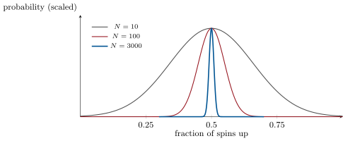
$N$ independent spins, each up or down: $2^N$ microstates. The macrostate “ $n$ up” has multiplicity $\Omega(n) = \binom Nn$ , overwhelmingly peaked at $n = N/2$ with relative width $\sim1/\sqrt N$ . For $N = 100$ : the all-up state is one; the balanced macrostate holds $1 \times 10^{29}$ . For $N = 10^{20}$ , deviations of even $10^{-8}$ in the up-fraction are suppressed by factors like $\eu^{-10^4}$ : the system is at its peak, and what we call equilibrium is the macrostate with the most microstates.

The multiplicity of the spin system against its up-fraction, for growing N: the peak sharpens as 1/√ N. At N 1020 the “distribution” is, for every practical purpose, a single value — macroscopic definiteness out of microscopic democracy. — The multiplicity of the spin system against its up-fraction, for growing $N$ : the peak sharpens as $1/\sqrt N$ . At $N \sim 10^{20}$ the “distribution” is, for every practical purpose, a single value — macroscopic definiteness out of microscopic democracy.

16.2 Entropy is a count

Definition 16.4 (Boltzmann entropy)

The statistical entropy of a macrostate is

S = k_{\text{B}}\ln\Omega , \qquad k_{\text{B}} = 1.38 \times 10^{-23}\,\mathrm{J}/\mathrm{K} .

The logarithm makes entropy additive where multiplicities multiply: for independent systems $\Omega = \Omega_1\Omega_2$ and $S = S_1 + S_2$ ; Boltzmann’s constant calibrates the count to the kelvin-and-joule units thermodynamics had already chosen. This $S$ , we will verify, is the entropy of the Year 1 volume’s second law — now with a microscopic meaning: entropy measures, in logarithmic currency, how many ways the macrostate can be realised.

Proposition 16.5 (Entropy of the ideal gas)

Counting the quantum states of $N$ identical atoms in a box (Proposition 7.5, one cell of $h^3$ per atom in phase space, divided by $N!$ for identity — Exercise 14.10) gives

S = Nk_{\text{B}}\Big[\ln\Big(\frac VN\,\frac1{\lambda_T^3}\Big) + \frac52\Big] , \qquad \lambda_T = \frac{h}{\sqrt{2\pi mk_{\text{B}}T}}

(the Sackur–Tetrode formula; $\lambda_T$ , the thermal de Broglie wavelength, is the size of an atom’s wave packet at temperature $T$ ). Two remarkable audits: the formula is extensive only thanks to the $N!$ ; and its absolute value — including the $h$ — matches calorimetric entropies of real gases (Exercise 16.11): classical thermodynamics, measured in the nineteenth century, already knew Planck’s constant without knowing it.

Proof. Admitted at this level. ∎

16.3 Temperature is a derivative of counting

Theorem 16.6 (Equilibrium and temperature)

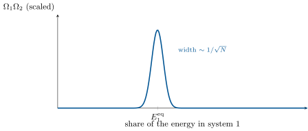
Let two systems exchange energy, the total $E = E_1 + E_2$ fixed. The joint multiplicity $\Omega_1(E_1)\,\Omega_2(E - E_1)$ is maximal — overwhelmingly so — at the partition where

\frac{\partial S_1}{\partial E_1} = \frac{\partial S_2}{\partial E_2} .

Defining

\frac1T = \frac{\partial S}{\partial E}\bigg|_{V,N} ,

equilibrium is equality of temperature, and energy flows spontaneously from high $T$ to low $T$ because that direction increases the total count. The same logic applied to volume and particle exchange yields $P/T = \partial S/\partial V$ and $-\mu/T = \partial S/\partial N$ : all of thermodynamics’ intensive quantities are derivatives of the count.

Proof. Maximise $\ln\Omega_1 + \ln\Omega_2$ over $E_1$ : the stationarity condition is the stated equality. Sharpness: the peak’s width is $\sim E/\sqrt N$ (Exercise 16.7), so the maximum is the observed state. If $\partial S_1/\partial E_1 > \partial S_2/\partial E_2$ , moving energy into 1 raises $S_{\text{tot}}$ : the colder body (larger $\partial S/\partial E$ ) absorbs — heat flows hot to cold as a counting statement. Check on the ideal gas: $S \propto \tfrac32 Nk_{\text{B}}\ln E + \cdots$ gives $1/T = \tfrac32 Nk_{\text{B}}/E$ , i.e. $E = \tfrac32 Nk_{\text{B}}T$ — the kinetic-theory result of the Year 1 volume, recovered from pure counting. ∎

Two systems sharing energy: the joint count against the split. The equilibrium partition — equal temperatures — is not merely the likeliest; for macroscopic N it is the only one ever observed. — Two systems sharing energy: the joint count against the split. The equilibrium partition — equal temperatures — is not merely the likeliest; for macroscopic $N$ it is the only one ever observed.

16.4 The second law, and stranger things

Proposition 16.7 (Irreversibility is arithmetic)

A constraint released (a wall removed, a valve opened) can only enlarge the accessible count: $\Omega$ grows, $S$ grows — the second law of the Year 1 volume, now as a statement about probability. Reversals are not forbidden but discounted: a gas of $N$ molecules re-gathering into the left half has probability $2^{-N}$ , and for one cubic centimetre of air the waiting time exceeds the age of the universe by a factor with $10^{19}$ digits. The arrow of time, at this level, is the direction in which counts increase.

Partial proof. Removing a constraint makes every formerly accessible microstate still accessible and adds new ones: $\Omega$ cannot decrease. The free-expansion count: each molecule doubles its accessible volume, $\Omega \to 2^N\Omega$ , so $\Delta S = Nk_{\text{B}}\ln2$ — exactly the thermodynamic result for isothermal free doubling. ∎

Example 16.8 (Negative temperature)

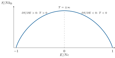
A system whose energy is bounded above — $N$ spins in a field, energy from $-N\epsilon$ to $+N\epsilon$ — has $\Omega(E)$ rising then falling: beyond the balanced point, adding energy reduces the count. There $\partial S/\partial E < 0$ : the temperature is negative. Such states exist (population inversions — the working state of every laser medium — and spin systems prepared by field reversal) and they are not cold but hotter than every positive temperature: energy flows from any $T < 0$ body into any $T > 0$ body. The honest ordering of temperatures runs $+0, \dots, +\infty \equiv -\infty, \dots, -0$ : what $1/T$ orders naturally, $T$ garbles (Exercise 16.9).

Entropy of the two-level spin system against energy. On the rising flank temperature is positive; at the crest it passes through infinity; on the falling flank — population inverted — it is negative, and hotter than anything on the left.

Method 16.9 (Microcanonical craft)

(1) Enumerate: what is a microstate here, and what does the macrostate fix? (2) Count $\Omega$ — combinatorics for discrete units, phase-space volume over $h^{3N}N!$ for gases. (3) Take the logarithm early: Stirling ( $\ln N! \approx N\ln N - N$ ) turns products into tractable sums. (4) Differentiate $S$ : energy derivative for $T$ , volume for $P$ , number for $\mu$ ; length or magnetisation derivatives for tensions and fields (Problem 16.1). (5) Trust the peak: fluctuations are down by $1/\sqrt N$ , so replace “most probable” by “equals” and apologise to no one.

Smoke stirred in a box, cut by a laser sheet: micro-motion beyond any bookkeeping, statistics taking over — the moment a mechanics problem becomes an entropy problem.

16.5 Exercises

Exercise 16.1 ★

Four spins. (a) List the multiplicities $\Omega(n)$ of the macrostates “ $n$ up”. (b) The probability of each macrostate under the postulate. (c) The entropy (in units of $k_{\text{B}}$ ) of each. (d) Which macrostate is “equilibrium”, and how bad an approximation is “the system is surely there” at $N = 4$ ?

Solution

Solution of Exercise 16.1.

(a) $1, 4, 6, 4, 1$ . (b) Over $16$ : $6.25\%$ , $25\%$ , $37.5\%$ , $25\%$ , $6.25\%$ . (c) $S/k_{\text{B}} = 0$ , $\ln4$ , $\ln6$ , $\ln4$ , $0$ . (d) $n = 2$ , holding only $37.5\%$ of the probability: at $N = 4$ , “equilibrium” is merely a plurality — the sharpness that licenses thermodynamics is bought with large $N$ .

Exercise 16.2 ★

Stirling in practice. (a) Compare $\ln N!$ with $N\ln N - N$ for $N = 10$ and $N = 100$ (use $\ln10! = 15.10$ , $\ln100! = 363.7$ ). (b) Show the relative error falls like $\ln N/N$ . (c) Use Stirling to show $\ln\binom N{N/2} \approx N\ln2 - \tfrac12\ln N +$ const. (d) Why is dropping the $\tfrac12\ln N$ utterly safe in a mole?

Solution

Solution of Exercise 16.2.

(a) $N = 10$ : $13.0$ against $15.1$ ( $14\%$ off); $N = 100$ : $360.5$ against $363.7$ ( $0.9\%$ ). (b) The neglected term is $\tfrac12\ln(2\pi N)$ : relative error $\sim\ln N/N$ . (c) Apply Stirling to the three factorials. (d) At $N = 10^{23}$ the dropped term is $\sim26$ against $N\ln2 \sim 10^{23}$ : twenty-two orders below the leading one.

Exercise 16.3 ★

(a) Show that for two independent systems $S = S_1 + S_2$ . (b) A system’s $\Omega$ doubles: by how much does $S$ rise — and what physical act (Proposition 16.7) does that correspond to for one particle? (c) Compute the entropy, in $k_{\text{B}}$ and in J/K, of a shuffled deck of 52 cards ( $\ln52! \approx 156.4$ ). (d) Why is card entropy thermodynamically negligible while molecular entropy is not?

Solution

Solution of Exercise 16.3.

(a) $\ln(\Omega_1\Omega_2) = \ln\Omega_1 + \ln\Omega_2$ . (b) $\Delta S = k_{\text{B}}\ln2$ — one particle offered a doubled volume. (c) $S = 156\,k_{\text{B}} = 2.2 \times 10^{-21}\,\mathrm{J}/\mathrm{K}$ . (d) Thermodynamic entropies carry factors of $10^{23}$ : all the shuffling in every casino on Earth is invisible next to a breath of warm air.

Exercise 16.4 ★

Free expansion, audited. One mole doubles its volume into vacuum. (a) $\Delta S$ from the counting argument. (b) The probability of observing the gas back in the original half. (c) Estimate the time scale for such a fluctuation given molecular rearrangement times of $10^{-10}\,\mathrm{s}$ — and compare with the age of the universe ( $4 \times 10^{17}\,\mathrm{s}$ ). (d) In what precise sense is the second law “only” probabilistic?

Solution

Solution of Exercise 16.4.

(a) $\Delta S = N_{\text{A}}k_{\text{B}}\ln2 = R\ln2 = 5.76\,\mathrm{J}/\mathrm{K}$ . (b) $2^{-N_{\text{A}}} \sim 10^{-1.8\times 10^{23}}$ . (c) Even sampling configurations every $10^{-10}\,\mathrm{s}$ , the expected wait dwarfs $4 \times 10^{17}\,\mathrm{s}$ by a factor whose exponent has twenty-three digits. (d) Not impossible — unwitnessable: the law is probabilistic in principle and absolute in any world that contains observers with finite patience.

Exercise 16.5 ★★

Ideal-gas counting. Starting from $\Omega \propto \dfrac{V^N}{N!\,h^{3N}}\times$ (momentum-shell volume $\propto E^{3N/2}$ ): (a) show $S = Nk_{\text{B}}[\ln V + \tfrac32\ln E] - k_{\text{B}}\ln N! +$ const. (b) Show that without the $N!$ , doubling the system (both $V$ and $N$ ) would not double $S$ — the extensivity failure of Exercise 14.10. (c) With Stirling, put the result in the form $S = Nk_{\text{B}}[\ln(V/N) + \tfrac32\ln(E/N)] +$ const $\cdot N$ . (d) Which physical inputs fixed the two “consts” history left undetermined (quantum cell size; particle identity)?

Solution

Solution of Exercise 16.5.

(a) Take the logarithm of the product. (b) Doubling $V, N$ at fixed $E/N$ : without $N!$ , $S$ gains an extra $N\ln2$ -type excess — the Gibbs failure. (c) Stirling on $\ln N!$ delivers the $V/N$ and $E/N$ combinations. (d) Planck’s cell $h^3$ fixes the entropy’s zero; identity of particles fixes the $N!$ — two quantum inputs hiding in classical thermodynamics.

Exercise 16.6 ★★

Thermodynamics from derivatives. Using the form of Exercise 16.5(c): (a) compute $1/T = \partial S/\partial E$ and recover $E = \tfrac32 Nk_{\text{B}}T$ ; (b) compute $P/T = \partial S/\partial V$ and recover $PV = Nk_{\text{B}}T$ ; (c) derive the adiabatic invariant: at constant $S$ and $N$ , show $VE^{3/2}$ is fixed, i.e. $TV^{2/3}$ — and match to the $PV^{5/3}$ of the Year 1 volume; (d) state what has been achieved: which empirical laws just became theorems of counting.

Solution

Solution of Exercise 16.6.

(a) $1/T = \tfrac32 Nk_{\text{B}}/E$ . (b) $P/T = Nk_{\text{B}}/V$ : the ideal-gas law, from counting. (c) Constant $S$ : $\ln(V/N) + \tfrac32\ln(E/N)$ fixed, so $VE^{3/2}$ constant; with $E \propto T$ : $TV^{2/3}$ constant, equivalent to $PV^{5/3}$ . (d) The gas law, the energy–temperature relation and the adiabatic exponent — three empirical pillars of the Year 1 volume — are now theorems.

Exercise 16.7 ★★

Sharpness of equilibrium. Two equal ideal-gas blocks share total energy $E$ . (a) Show $\ln[\Omega_1\Omega_2]$ is maximal at the even split. (b) Expand to second order in the imbalance $x = (E_1 - E_2)/E$ and show the probability is $\propto\eu^{-3Nx^2/4}$ (each block $\tfrac32 N$ degrees of freedom — keep factors loose). (c) For $N = 10^{22}$ : the r.m.s. imbalance. (d) The temperature difference that imbalance represents, for gas at $300\,\mathrm{K}$ : could any thermometer see it?

Solution

Solution of Exercise 16.7.

(a) Symmetry (equal blocks). (b) Each $\ln\Omega \propto \tfrac32 N\ln E_i$ : expanding about the even split gives a Gaussian in $x$ of variance $\sim1/N$ . (c) $x_{\text{rms}} \sim 10^{-11}$ . (d) $\Delta T/T \sim x_{\text{rms}}$ : nano-nanokelvins — fluctuations exist, and are unmeasurably tame at laboratory scale.

Exercise 16.8 ★★

The two-level (Schottky) solid: $N$ sites, each of energy $0$ or $\epsilon$ ; $n$ excited. (a) $\Omega(n)$ and $S(n)$ . (b) With $E = n\epsilon$ and Stirling, derive

\frac1T = \frac{k_{\text{B}}}{\epsilon}\, \ln\frac{N - n}{n} , \qquad\text{hence}\qquad \frac nN = \frac{1}{\eu^{\epsilon/k_{\text{B}}T} + 1} .

(c) Sketch $E(T)$ and the heat capacity: a bump (the Schottky anomaly) near $k_{\text{B}}T \sim \epsilon/2$ — why does $C$ vanish at both ends? (d) Where has the occupation formula’s shape appeared before, and where will it return (Chapter 19)?

Solution

Solution of Exercise 16.8.

(a) $\Omega = \binom Nn$ , $S = k_{\text{B}}\ln\binom Nn$ . (b) $1/T = \partial S/\partial E = (k_{\text{B}}/\epsilon)[\ln(N-n) - \ln n]$ ; solve for $n/N$ . (c) $E(T)$ rises from $0$ to the saturation $N\epsilon/2$ ; $C = \dd E/\dd T$ vanishes at low $T$ (no quantum can be afforded) and at high $T$ (both levels equally full, nothing left to absorb): a bump between — the calorimetric fingerprint of any two-level population, used to find magnetic impurities in solids. (d) It is the thermal two-level occupation — and, with $\epsilon \to E - \mu$ , it will reappear verbatim as the Fermi–Dirac distribution.

Exercise 16.9 ★★

Below zero. For the spin system of Example 16.8 with level splitting $\epsilon$ : (a) show $T < 0$ exactly when more than half the spins are up (population inverted). (b) Compute $T$ for a 60:40 inversion with $\epsilon = 10^{-4}\,\mathrm{eV}$ . (c) Show energy always flows from negative- $T$ to positive- $T$ bodies (compare $\partial S/\partial E$ ). (d) Why can a system with unbounded energy (a gas) never reach $T < 0$ ?

Solution

Solution of Exercise 16.9.

(a) $1/T \propto \ln[(N-n)/n] < 0$ exactly when $n > N/2$ . (b) $T = \epsilon/[k_{\text{B}}\ln(2/3)] = -2.9\,\mathrm{K}$ . (c) A negative- $T$ body gains entropy by losing energy, a positive- $T$ body gains by receiving: both counts grow when energy flows negative $\to$ positive — the inverted system is the universal donor, i.e. hotter than everything. (d) With unbounded energy, $\Omega(E)$ never turns over: $\partial S/\partial E$ stays positive at any finite energy.

Exercise 16.10 ★★★

Mixing, quantitatively. Two different gases ( $N$ each, volumes $V$ ) are joined. (a) Compute $\Delta S$ by counting. (b) Same gas: show, $N!$ ’s included, $\Delta S = 0$ . (c) Helium-3 and helium-4 are different: joining them does create $2Nk_{\text{B}}\ln2$ — yet no heat flows and no work is done: where is the entropy increase physically (what would separating them again cost)? (d) The minimum work to re-separate at temperature $T$ : express it, and name the modern industry built on paying it (isotope separation).

Solution

Solution of Exercise 16.10.

(a) Each gas doubles its accessible volume: $\Delta S = 2Nk_{\text{B}}\ln2$ . (b) The $N!$ ’s of the merged populations exactly absorb the apparent gain: $\Delta S = 0$ . (c) The entropy increase is the loss of sortedness: no macroscopic variable moved, but re-separating now requires work — the increase is stored as a future bill. (d) $W_{\min} = T\Delta S = 2Nk_{\text{B}}T\ln2$ ; isotope-separation plants (uranium centrifuge cascades, helium-3 recovery) pay this thermodynamic minimum many times over in practice.

Exercise 16.11 ★★★

The tables knew about $h$ . Sackur–Tetrode for argon ( $m = 6.6 \times 10^{-26}\,\mathrm{kg}$ ) at $300\,\mathrm{K}$ , $1\,\mathrm{bar}$ ( $V/N = k_{\text{B}}T/P$ ): (a) compute $\lambda_T$ ; (b) compute $S/N k_{\text{B}}$ ; (c) compare with the calorimetric value $S_{\text{molar}} = 154.8\,\mathrm{J}/(\mathrm{mol}\,\mathrm{K})$ , i.e. $S/Nk_{\text{B}} = 18.6$ ; (d) explain what is being tested: which two quantum inputs sit inside a number measured with ice calorimeters before 1912?

Solution

Solution of Exercise 16.11.

(a) $\lambda_T = 1.6 \times 10^{-11}\,\mathrm{m}$ . (b) $V/N = k_{\text{B}}T/P = 4.1 \times 10^{-26}\,\mathrm{m}^{3}$ : $V/N\lambda_T^3 = 1.0 \times 10^{7}$ , so $S/Nk_{\text{B}} = \ln(1.0 \times 10^{7}) + 2.5 = 18.6$ . (c) Dead on the calorimetric $18.6$ . (d) The absolute entropy contains $h$ (through $\lambda_T$ ) and the $N!$ : heat measurements from the age of steam confirm, to three digits, the quantum of action and the identity of atoms.

Exercise 16.12 ★★★

Fluctuations you can see. The number of molecules in a small volume $v$ of gas fluctuates; the probability of a relative deviation $\delta$ is $\propto\eu^{-\bar n\delta^2/2}$ ( $\bar n = Nv/V$ — accept this Gaussian, or derive from the binomial). (a) For $v$ a cube of side $550\,\mathrm{nm}$ at atmospheric density: $\bar n$ and the r.m.s. $\delta$ . (b) Why are these permanent few-per-mille density ripples at optical scales exactly what Problem 13.1 needed to let air scatter at all? (c) At what $\bar n$ (hence what scale) would fluctuations reach $10\%$ ? (d) Close the loop in one sentence: the blue of the sky is a statement about $\sqrt N$ statistics.

Solution

Solution of Exercise 16.12.

(a) $v = (550\,\mathrm{nm})^3 = 1.7 \times 10^{-19}\,\mathrm{m}^{3}$ : $\bar n = 4.2 \times 10^{6}$ , $\delta_{\text{rms}} = 1/\sqrt{\bar n} \approx 5 \times 10^{-4}$ . (b) A perfectly uniform medium would scatter nothing sideways (Problem 13.1, Part III): these irreducible $\sqrt N$ ripples in every optical cell are precisely the disorder that lets the sky exist. (c) $\bar n = 100$ : $v \approx (16\,\mathrm{nm})^3$ . (d) The sky is blue because air is made of countable molecules whose numbers fluctuate as $\sqrt N$ — Einstein used exactly this to argue molecules were real.

16.6 Problem: The entropic spring

Problem 16.1

Weekend problem — why rubber pulls back

Stretch a rubber band and it snaps back — yet its molecules’ bonds are barely deformed and its internal energy barely changes. Rubber’s restoring force is not energy seeking a minimum but entropy seeking a maximum: the first great victory of pure counting over mechanism, with the same mathematics running today’s single-molecule DNA experiments. Model: a chain of $N$ rigid links, each of length $b$ , each pointing left or right along the pull axis; end-to-end extension $x = (n_+ - n_-)\,b$ .

Part I — Counting configurations.

Express $n_\pm$ in terms of $N$ and $x$ , and write the multiplicity $\Omega(x)$ .
Where is $\Omega$ maximal, and what does that say about a free chain’s preferred extension?
With Stirling, show for $x \ll Nb$ :

$S(x) \approx S(0) - \frac{k_{\text{B}}x^2}{2Nb^2} .$
The chain’s energy is (in this model) independent of $x$ : justify calling any restoring force “entropic”.
The r.m.s. extension of the free chain is $b\sqrt N$ (random walk): for $N = 10^4$ and $b = 0.5\,\mathrm{nm}$ , compare the coil size with the stretched length $Nb$ .
Real rubber is a network of such chains between cross-links: which single parameter of the model does vulcanisation (more cross-links) change?

Part II — The force of counting.

For a system held at temperature $T$ , the tension required to hold extension $x$ is $f = -T\,\partial S/\partial x$ (accept this from $\dd E = T\dd S + f\dd x$ at constant energy): derive

$f = \frac{k_{\text{B}}T\,x}{Nb^2} .$
Hooke’s law has emerged with spring constant $k = k_{\text{B}}T/Nb^2$ : evaluate it for one chain with $N = 10^{4}$ , $b = 0.5\,\mathrm{nm}$ at $300\,\mathrm{K}$ .
The startling factor is $T$ : what should a rubber band under fixed load do when heated? Contrast with a steel spring.
Estimate the force to stretch one chain to half its full length, and the force scale $k_{\text{B}}T/b$ at which the linear model fails.
A rubber band of cross-section $1\,\mathrm{mm}^{2}$ contains $\sim10^{14}$ effective chains in parallel: estimate its spring constant and compare with experience.
Why does rubber stiffen (not soften) with temperature, gram for gram, while metals soften?

Part III — The Gough–Joule kitchen.

Stretch a rubber band quickly (adiabatically) against your lip: it warms. Explain with the entropy budget: stretching reduces configurational entropy, so where must entropy (heat) go at constant total?
Release it quickly: it cools. Complete the symmetric argument.
A weighted rubber band is gently heated (hair dryer): which way does the weight move, and why is this the clean signature of entropic elasticity?
Design the counter-experiment with a steel spring: what happens instead, and why (which kind of elasticity)?
An engine: a wheel with rubber spokes, heated on one side, turns steadily. Trace one cycle’s logic (heated spokes contract, unbalancing the wheel).
The same $f = k_{\text{B}}Tx/Nb^2$ law, measured by optical tweezers on single DNA molecules (with $b \approx 100\,\mathrm{nm}$ , $N \approx 500$ for a bacterial genome fragment), gives forces in which range? (Compute $k_{\text{B}}T/b$ .) Why did this make the model directly testable on one molecule?

Part IV — The moral.

The chain model has no interactions and no energy scale, yet produces a force law: state precisely where the force “comes from” in the microcanonical language of this chapter.
Why does the force vanish at $T = 0$ — and what does that say about the nature of elasticity in a world without thermal agitation?
Compare the entropic spring constant’s $T$ -linearity with the ideal-gas pressure’s $T$ -linearity: show both are the same phenomenon (counting configurations against a constraint) in different clothes.
The heated band lifts a weight, doing real work: trace the energy’s source and route (heat in from the dryer, entropy bookkeeping, work out) and confirm the first law is untouched.
The ideal chain ignores self-avoidance and link-bending energy: name one measured feature of real rubber each omission hides (sharp stiffening near full extension; strain-induced crystallisation and hysteresis).
Proteins fold, membranes flicker, polymers coil: why is $k_{\text{B}}T$ at body temperature the natural force currency ( $k_{\text{B}}T/\mathrm{nm}$ in piconewtons — compute it) of all soft and living matter?
Summarise the named result: a chain of $10^4$ blind links, counted honestly, yields Hooke’s law with $k = k_{\text{B}}T/Nb^2$ , predicts that rubber warms when stretched and lifts weights when heated — entropy acting as a force, verified from bicycle inner tubes to single DNA molecules at $\sim0.04\,\mathrm{pN}$ scales.

Solution

Solution of Problem 16.1.

1. $n_\pm = \tfrac12(N \pm x/b)$ ; $\Omega = N!/n_+!\,n_-!$ . 2. At $x = 0$ : the free chain coils; full extension has $\Omega = 1$ . 3. Stirling on the binomial, expanded to second order in $x/Nb$ : the stated Gaussian entropy. 4. With $E$ independent of $x$ , any pull toward small $x$ can only come from the count: entropic by construction. 5. Coil $\sim b\sqrt N = 50\,\mathrm{nm}$ against $Nb = 5\,\text{µ}\mathrm{m}$ : the free chain is a hundred times shorter than its contour — crumpled almost entirely. 6. $N$ , the number of links between cross-links: vulcanisation shortens the effective chains, stiffening the network. 7. $f = -T\,\partial S/\partial x = k_{\text{B}}Tx/Nb^2$ . 8. $k = k_{\text{B}}T/Nb^2 = 4.14 \times 10^{-21}/(10^{4} \times 2.5 \times 10^{-19}) = 1.7 \times 10^{-6}\,\mathrm{N}/\mathrm{m}$ per chain. 9. $k \propto T$ : heated under fixed load, the band stiffens and contracts, lifting the load; a steel spring merely softens and sags a little. 10. $f(Nb/2) = k_{\text{B}}T/2b \approx 4\,\mathrm{pN}$ ; the linear law fails as $f$ approaches $k_{\text{B}}T/b \approx 8\,\mathrm{pN}$ , where the chain nears full extension. 11. $\sim10^{14}$ chains in parallel and $\sim10^{5}$ coil-lengths in series along a centimetre: $k_{\text{band}} \sim k_{\text{chain}} \times 10^{14}/10^{5} \sim 10^{2}$ – $10^{3}\,\mathrm{N}/\mathrm{m}$ — the familiar feel of a rubber band. 12. Rubber’s stiffness is $k_{\text{B}}T$ per configuration: more agitation, more recoil; metallic stiffness is bond energy, which anharmonic agitation loosens. 13. Stretching cuts the configurational count; done fast (no entropy exchanged with outside), the lost configurational entropy must reappear as thermal entropy: the band warms — $1\,\mathrm{K}$ -scale, lip-detectable. 14. Releasing restores configurations; the thermal account refunds the difference: it cools. 15. The weight rises: contraction on heating is the entropic signature (energy-elastic materials expand). 16. The steel spring lengthens slightly (thermal expansion) and its modulus drops: opposite sign — elasticity of energy, not of counting. 17. Heated spokes contract, pulling the rim’s mass off-centre toward the cool side; gravity torques the unbalanced wheel; each spoke re-relaxes as it rotates away: a heat engine whose working substance is entropy itself. 18. $k_{\text{B}}T/b = 4.14 \times 10^{-21}/10^{-7} = 4 \times 10^{-14}\,\mathrm{N} = 0.04\,\mathrm{pN}$ : piconewtons and below — exactly the optical-tweezer range, so the force–extension law of one DNA molecule could be traced point by point (and matched, with the refinements of item 23). 19. From nowhere but the count: at extension $x$ there are fewer microstates than at $x - \dd x$ , and thermal agitation drifts the chain toward the bigger count; the “force” is $T$ times the entropy gradient. 20. At $T = 0$ nothing explores configurations: the entropic force vanishes with the agitation that powers it — elasticity would be purely energetic, and rubber would behave like a limp thread. 21. Gas: $P = T\,\partial S/\partial V$ with $S \ni Nk_{\text{B}}\ln V$ ; chain: $f = -T\,\partial S/\partial x$ with the Gaussian count — both are counting pushed against a constraint, priced at $T$ . 22. The dryer’s heat enters the band; part is converted to work in the isothermal contraction, the books balanced by the entropy carried in and out — a miniature heat engine, first law intact. 23. Finite extensibility (the real force diverges near full stretch — the worm-like-chain refinement) and strain-induced crystallisation (alignment orders the chains, giving hysteresis and heat release beyond the ideal model). 24. $k_{\text{B}}T/\mathrm{nm} = 4.1\,\mathrm{pN}$ : the force at which thermal energy and nanometre displacements trade evenly — molecular motors, folding proteins and stretched DNA all operate within an order of magnitude of it. 25. Ten thousand blind links, counted: Hooke’s law with $k = k_{\text{B}}T/Nb^2$ , warmth on stretching, weights lifted by hot air, and single molecules obeying at $0.04\,\mathrm{pN}$ — entropy, acting as a force.

Terms defined in this chapter

See all 431 terms in the glossary