University Physics — Year 3 · Bachelor Year 3

18The Grand Canonical Ensemble

A drop of water in humid air neither grows nor shrinks; oxygen binds to haemoglobin in the lungs and unbinds in the muscles; a battery drives electrons through a phone because they are “more expensive” in one electrode than the other. In each case the currency being balanced is not temperature but the chemical potential $\mu$ : the free-energy cost of one more particle. This chapter opens the second reservoir valve — particles as well as energy — and builds the grand canonical ensemble, whose reward is astonishing efficiency: the occupation of a single quantum level, fermion or boson, follows in two lines, and with it the master formulas of the next chapter. Its applications run from the adsorption isotherms of gas masks and catalytic converters to the Saha equation, with which a Harvard doctoral student in 1925 read the temperatures of the stars and discovered, against all expectation, that the universe is made of hydrogen.

18.1 Particles join the negotiation

Theorem 18.1 (Grand canonical distribution)

A system exchanging energy and particles with a reservoir at temperature $T$ and chemical potential $\mu$ occupies its state $s$ (energy $E_s$ , particle number $N_s$ ) with probability

\mathcal P_s = \frac{\eu^{-\beta(E_s - \mu N_s)}}{\Xi} , \qquad \Xi = \sum_s\eu^{-\beta(E_s - \mu N_s)} ,

the grand partition function. From $\Xi$ : $\langle N\rangle = k_{\text{B}}T\,\partial\ln\Xi/\partial\mu$ , and the grand potential $\Phi = -k_{\text{B}}T\ln\Xi$ obeys $\Phi = -PV$ .

Partial proof. As in Theorem 17.1, expand the reservoir’s entropy in both withdrawals: $S_{\text{res}}(E - E_s, N - N_s) \approx S_{\text{res}} - E_s/T + \mu N_s/T$ , using $\partial S/\partial N = -\mu/T$ (Theorem 16.6). The averages follow by differentiation; $\Phi = -PV$ is admitted (it follows from extensivity). ∎

Definition 18.2 (What $\mu$ means)

$\mu$ is the cost, in free energy, of adding one particle at fixed $T$ and $V$ . Particles flow spontaneously from high $\mu$ to low $\mu$ — diffusion, osmosis, evaporation, chemical reactions and electric currents are all $\mu$ -gradients relaxing. At equilibrium between any two phases or places, $\mu$ is equal on both sides — the third equality (with $T$ and $P$ ) that governs coexistence. For a classical ideal gas,

\mu = k_{\text{B}}T\,\ln\!\big(n\lambda_T^3\big) < 0 \quad\text{(dilute gas)} :

adding a particle to a dilute gas lowers the free energy, because the entropy gain outweighs any energy cost — the sign that drives evaporation into dry air. And a battery is a $\mu$ -machine: its voltage is the chemical-potential drop per electron between its electrodes, $U = \Delta\mu/e$ — volts are electron chemistry’s exchange rate, which is why cells deliver single-digit volts.

18.2 One level at a time: the master trick

Theorem 18.3 (Occupation of a single quantum level)

Take as “the system” one single-particle level of energy $\epsilon$ , in grand contact with the gas of all the others. Fermions (occupancy $0$ or $1$ ):

\Xi = 1 + \eu^{-\beta(\epsilon - \mu)} \;\Longrightarrow\; \bar n_{\text{FD}} = \frac{1}{\eu^{\beta(\epsilon - \mu)} + 1} .

Bosons (occupancy $0, 1, 2, \dots$ ):

\Xi = \frac{1}{1 - \eu^{-\beta(\epsilon - \mu)}} \;\Longrightarrow\; \bar n_{\text{BE}} = \frac{1}{\eu^{\beta(\epsilon - \mu)} - 1} ,

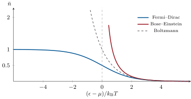
requiring $\mu < \epsilon_{\min}$ . Both reduce to the Boltzmann factor $\eu^{-\beta(\epsilon - \mu)}$ when occupations are rare. These two formulas, obtained in two lines each, are the entire input of quantum statistics: the next chapter is their harvest.

Proof. Fermions: two terms. Bosons: a geometric series, convergent only for $\mu < \epsilon$ . In both cases $\bar n = k_{\text{B}}T\, \partial\ln\Xi/\partial\mu$ gives the stated forms. ∎

The three occupation laws against ( - )/k_ BT: fermions saturate at one per state (a smoothed step at =), bosons pile up without bound as , and both join the dilute Boltzmann tail on the right — the classical regime is where a state is rarely visited at all. — The three occupation laws against $(\epsilon - \mu)/k_{\text{B}}T$ : fermions saturate at one per state (a smoothed step at $\epsilon = \mu$ ), bosons pile up without bound as $\epsilon \to \mu$ , and both join the dilute Boltzmann tail on the right — the classical regime is where a state is rarely visited at all.

18.3 Adsorption: sites for rent

Proposition 18.4 (The Langmuir isotherm)

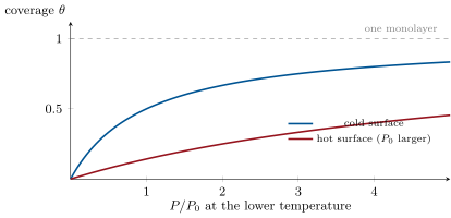
A surface offers independent sites, each empty or holding one gas molecule with binding energy $-\epsilon_0$ ; the gas above, at pressure $P$ , is the reservoir. Each site is a two-state grand system, and its occupation is

\theta = \frac{1}{\eu^{\beta(-\epsilon_0 - \mu)} + 1} = \frac{P}{P + P_0(T)} , \qquad P_0(T) = \frac{k_{\text{B}}T}{\lambda_T^3}\, \eu^{-\epsilon_0/k_{\text{B}}T} ,

using the ideal-gas $\mu$ . Coverage rises linearly at low pressure and saturates at one monolayer — the Langmuir isotherm, the working curve of catalytic converters, activated charcoal, gas masks and the oxygen-binding of blood (Exercise 18.6). The crossover pressure $P_0$ falls exponentially with binding energy and rises steeply with temperature: heating a surface shakes its guests loose — why baking glassware under vacuum is how one truly cleans it.

Proof. The site’s occupation is Theorem 18.3 (fermionic form: a site holds at most one) with $\epsilon = -\epsilon_0$ ; substitute $\eu^{\beta\mu} = n\lambda_T^3 = P\lambda_T^3/k_{\text{B}}T$ . ∎

Langmuir isotherms: coverage against pressure, saturating at a monolayer. Heat the surface and the same coverage demands far more pressure — adsorption is a negotiation the hot surface keeps losing. — Langmuir isotherms: coverage against pressure, saturating at a monolayer. Heat the surface and the same coverage demands far more pressure — adsorption is a $\mu$ negotiation the hot surface keeps losing.

18.4 Ionisation equilibria: the Saha equation

Proposition 18.5 (Saha’s equation)

In a hot gas the reaction $\text{H} \rightleftharpoons \text{p} + \text{e}$ equilibrates when $\mu_{\text{H}} = \mu_{\text{p}} + \mu_{\text{e}}$ . Writing each $\mu$ with the ideal-gas form (the atom credited with its binding $-E_{\text{I}}$ ) gives

\frac{n_{\text{e}}\,n_{\text{p}}}{n_{\text{H}}} = \frac{1}{\lambda_{T,\text{e}}^3}\, \eu^{-E_{\text{I}}/k_{\text{B}}T} \qquad\Big(\lambda_{T,\text{e}} = h/\sqrt{2\pi m_{\text{e}}k_{\text{B}}T}\Big)

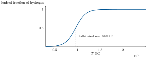
(up to spin-degeneracy factors of order one). Two competing currencies again: the Boltzmann factor taxes ionisation by $E_{\text{I}} = 13.6\,\mathrm{eV}$ , while the prefactor — the entropy of the freed electron, with its $\lambda_T^{-3}$ worth of accessible states — subsidises it. The subsidy is so large at stellar densities that hydrogen ionises appreciably already near $10\,000\,\mathrm{K}$ , where $k_{\text{B}}T$ is only $0.9\,\mathrm{eV}$ : equilibria are fought over free energy, not energy — and the stars’ spectra are the ledger (Problem 18.1).

Partial proof. Set $\mu_{\text{H}} = \mu_{\text{p}} + \mu_{\text{e}}$ with $\mu_i = k_{\text{B}}T\ln(n_i\lambda_{T,i}^3) + \varepsilon_i$ ( $\varepsilon_{\text{H}} = -E_{\text{I}}$ , the others zero); exponentiate. The proton’s and atom’s thermal wavelengths nearly cancel (equal masses); degeneracy factors are admitted. ∎

The Saha ionisation of hydrogen at photospheric density (schematic): a sharp transition near 10\,000\, K, far below the naive E_ I/k_ B 160\,000\, K — the freed electron’s entropy pays most of the bill. — The Saha ionisation of hydrogen at photospheric density (schematic): a sharp transition near $10\,000\,\mathrm{K}$ , far below the naive $E_{\text{I}}/k_{\text{B}} \approx 160\,000\,\mathrm{K}$ — the freed electron’s entropy pays most of the bill.

Method 18.6 (Grand canonical craft)

(1) Anything exchanging particles with a large partner: give the partner a $\mu$ and weight states by $\eu^{-\beta(E - \mu N)}$ . (2) Independent sites or levels factorise: solve one, multiply. (3) For a classical-gas reservoir, $\eu^{\beta\mu} = n\lambda_T^3$ converts $\mu$ to measurable pressure. (4) Reactions and phase changes: balance the $\mu$ ’s, one per species, binding energies included — expect entropy prefactors to shift equilibria far from naive Boltzmann guesses. (5) Electrons in solids: their $\mu$ is the Fermi level, and differences of $\mu$ are voltages — the bridge to Chapter 24.

18.5 Exercises

Exercise 18.1 ★

(a) Two boxes of the same gas at the same $T$ but different densities are connected: which way do particles flow, in $\mu$ -language? (b) Show from the ideal-gas $\mu$ that flow stops at equal densities. (c) Water sits under humid air: state the equilibrium condition in $\mu$ ’s. (d) Why does laundry dry even below $100\,^\circ$ C when the air is dry (compare $\mu$ ’s, not temperatures)?

Solution

Solution of Exercise 18.1.

(a) From the denser box to the thinner: from high $\mu = k_{\text{B}}T\ln(n\lambda_T^3)$ to low. (b) Equal $T$ makes $\lambda_T$ common: equal $\mu$ is equal $n$ . (c) $\mu_{\text{liquid}} = \mu_{\text{vapour}}$ — the definition of saturated humidity. (d) In dry air the vapour’s $\mu$ (low $n$ ) sits below the liquid’s: water evaporates down the $\mu$ -hill regardless of never boiling.

Exercise 18.2 ★

The chemical potential of air. (a) Compute $\lambda_T$ for N $_2$ at $300\,\mathrm{K}$ . (b) Compute $n\lambda_T^3$ at $1\,\mathrm{bar}$ and the resulting $\mu$ in eV. (c) Why is $\mu < 0$ no paradox (which term of $F = E - TS$ dominates on adding a molecule)? (d) At what density would $\mu$ reach zero, and what does $n\lambda_T^3 \sim 1$ herald (Exercise 18.11)?

Solution

Solution of Exercise 18.2.

(a) $\lambda_T = 1.9 \times 10^{-11}\,\mathrm{m}$ . (b) $n\lambda_T^3 = 1.7 \times 10^{-7}$ : $\mu = k_{\text{B}}T\ln(1.7 \times 10^{-7}) = -0.40\,\mathrm{eV}$ . (c) The entropy term: a new molecule opens $\sim1/n\lambda_T^3$ states, and $-TS$ wins over any kinetic cost. (d) $n = \lambda_T^{-3} \approx 1.5 \times 10^{32}\,\mathrm{m}^{-3}$ — thousands of times liquid density for air; $n\lambda_T^3 \sim 1$ is the border of quantum degeneracy (Exercise 18.11).

Exercise 18.3 ★

Derive the Fermi–Dirac occupation from its two-term $\Xi$ , step by step; check the limits $\epsilon \ll \mu$ , $\epsilon \gg \mu$ , and the value at $\epsilon = \mu$ . Where has this function already appeared in this book (Exercise 16.8)?

Solution

Solution of Exercise 18.3.

$\Xi = 1 + \eu^{-\beta(\epsilon-\mu)}$ ; $\bar n = k_{\text{B}}T\, \partial_\mu\ln\Xi = \eu^{-\beta(\epsilon-\mu)}/(1 + \eu^{-\beta(\epsilon-\mu)})$ , the stated form. Limits: $1$ deep below $\mu$ , Boltzmann tail far above, exactly $\tfrac12$ at $\epsilon = \mu$ . It is the thermal two-level occupation of the Schottky solid — the same curve, re-labelled.

Exercise 18.4 ★

Volts are chemistry. (a) A lithium cell holds $3.0\,\mathrm{V}$ : express the chemical-potential difference per electron in eV and per mole in kJ. (b) Why are all everyday batteries single-digit volts (what sets the scale of chemical $\mu$ differences)? (c) A lead–acid car battery stacks six cells: why stack rather than find a $12\,\mathrm{eV}$ reaction? (d) In $\mu$ -language, what is a battery doing when it is “flat”?

Solution

Solution of Exercise 18.4.

(a) $3.0\,\mathrm{eV}$ per electron; $\times N_{\text{A}}e$ : $\approx290\,\mathrm{kJ}/\mathrm{mol}$ . (b) Chemical potentials differ by bond energies — electron-volts: batteries inherit chemistry’s energy scale. (c) No chemical couple offers a $12\,\mathrm{eV}$ step (it would tear the electrolyte apart); series stacking adds $\mu$ -drops safely. (d) Its electrodes’ electron chemical potentials have equalised: no gradient, no push, however much matter remains.

Exercise 18.5 ★★

Bosons at a level. (a) Sum the geometric series for $\Xi$ and derive $\bar n_{\text{BE}}$ . (b) Why must $\mu$ stay below the lowest level — what diverges otherwise, and what does the divergence foreshadow (Chapter 19)? (c) Compute $\bar n$ for $(\epsilon - \mu)/k_{\text{B}}T = 0.1$ , $1$ , $3$ and compare with Boltzmann. (d) Photons have $\mu = 0$ : give the physical reason (their number is not conserved — walls absorb and emit freely).

Solution

Solution of Exercise 18.5.

(a) Geometric series with ratio $\eu^{-\beta(\epsilon-\mu)} < 1$ ; differentiate. (b) At $\mu \to \epsilon_{\min}$ the series diverges: the level can absorb unbounded population — the macroscopic pile-up that becomes Bose–Einstein condensation. (c) $\bar n = 9.51$ , $0.58$ , $0.052$ against Boltzmann’s $0.90$ , $0.37$ , $0.050$ : identical in the dilute tail, wildly enhanced near $\mu$ . (d) Since walls create and destroy photons at will, equilibrium cannot depend on their number: the free-energy cost of one more photon is zero, $\mu = 0$ .

Exercise 18.6 ★★

Langmuir at work. (a) From the isotherm, what pressure achieves $\theta = 0.5$ ? $0.9$ ? (b) Myoglobin binds O $_2$ on one site: saturation follows Langmuir in the oxygen partial pressure — why is a hyperbolic (not sigmoidal) curve observed for myoglobin but a cooperative S-curve for four-site haemoglobin? (c) Carbon monoxide binds to the same sites with $\epsilon_0$ larger by $\approx0.13\,\mathrm{eV}$ : at equal partial pressures and $310\,\mathrm{K}$ , compute the occupancy ratio CO:O $_2$ and explain CO poisoning. (d) Why does hyperbaric oxygen therapy work, in isotherm language?

Solution

Solution of Exercise 18.6.

(a) $P = P_0$ ; $P = 9P_0$ . (b) One independent site gives the hyperbola $P/(P + P_0)$ — myoglobin; haemoglobin’s four interacting sites load cooperatively, steepening the curve into the S shape that loads fully in the lungs and unloads in the tissues. (c) $\eu^{0.13/0.0267} \approx 130$ : at equal partial pressures CO wins the sites a hundredfold — a trace of CO evicts oxygen from the blood. (d) Raising the O $_2$ partial pressure raises its $\mu$ and re-tilts the competition: the isotherm is fought over $\mu$ ’s, and hyperbaric oxygen simply outbids.

Exercise 18.7 ★★

Number fluctuations. (a) Show $\operatorname{Var}N = k_{\text{B}}T\,\partial\langle N\rangle/\partial\mu$ . (b) For the classical ideal gas, deduce $\operatorname{Var}N = \langle N\rangle$ : Poisson. (c) Reconcile with the density fluctuations of Exercise 16.12. (d) For a single fermionic level, compute $\operatorname{Var}n = \bar n(1 - \bar n)$ : where are fermion numbers quietest, and why?

Solution

Solution of Exercise 18.7.

(a) Differentiate $\langle N\rangle = k_{\text{B}}T\,\partial_\mu \ln\Xi$ once more. (b) $\langle N\rangle \propto \eu^{\beta\mu}$ : $\partial_\mu\langle N\rangle = \beta\langle N\rangle$ , so $\operatorname{Var}N = \langle N\rangle$ . (c) The Gaussian with variance $\bar n$ of that exercise is this Poisson statement, seen in a sub-volume. (d) $\operatorname{Var}n = \bar n(1 - \bar n)$ : zero when the level is surely empty or surely full — Pauli blocking silences fluctuations deep in a Fermi sea.

Exercise 18.8 ★★

Osmosis from $\mu$ . A membrane passes water but not solute (concentration $c$ per volume, dilute). (a) Equating water’s $\mu$ across the membrane, show the pure-water side must be over-pressured by $\Pi = ck_{\text{B}}T$ (van ’t Hoff) — accept that dissolved solute lowers water’s $\mu$ by $-k_{\text{B}}T\,c/n_{\text{w}}$ per water molecule. (b) Compute $\Pi$ for physiological saline ( $c \approx 3 \times 10^{26}\,\mathrm{m}^{-3}$ total particles). (c) Red cells in pure water: which way does water flow, and with what result? (d) Why do trees need neither pumps nor miracles to raise sap tens of metres (osmotic and capillary $\mu$ -gradients)?

Solution

Solution of Exercise 18.8.

(a) Solute dilutes water’s entropy, lowering its $\mu$ ; pressure raises $\mu$ : balance fixes $\Pi = ck_{\text{B}}T$ . (b) $\Pi = 3 \times 10^{26} \times 1.38 \times 10^{-23} \times 310 \approx 1.3\,\mathrm{MPa}$ — thirteen atmospheres inside your veins, routinely balanced. (c) Pure water’s $\mu$ exceeds the cell interior’s: water floods in and the cells burst (haemolysis) — why infusions are saline, never pure water. (d) Root-to-leaf $\mu$ -gradients (solutes, evaporation at the leaf) pull water up as osmotic and capillary pressure differences: tens of metres without a single moving part.

Exercise 18.9 ★★

Equilibrium in a field. In gravity, equilibrium of a gas column requires the total chemical potential $\mu(h) = k_{\text{B}}T\ln(n\lambda_T^3) + mgh$ to be uniform. (a) Derive the barometric law from this in one line. (b) Generalise to a centrifuge at angular velocity $\omega$ (potential $-\tfrac12 m\omega^2r^2$ ) and obtain the radial profile. (c) Uranium enrichment centrifuges spin at $\omega r \sim 600\,\mathrm{m}/\mathrm{s}$ : compute the equilibrium ratio of $^{238}$ UF $_6$ to $^{235}$ UF $_6$ enhancement per stage, $\exp[\Delta m\,\omega^2 r^2/2k_{\text{B}}T]$ with $\Delta m = 5 \times 10^{-27}\,\mathrm{kg}$ , $T = 320\,\mathrm{K}$ . (d) Why are many stages cascaded?

Solution

Solution of Exercise 18.9.

(a) Uniform $\mu$ : $k_{\text{B}}T\ln n(h) + mgh =$ const, i.e. the barometric exponential. (b) $n(r) \propto \eu^{+m\omega^2r^2/2k_{\text{B}}T}$ : heavy species pile at the rim. (c) $\exp[\Delta m\,\omega^2r^2/2k_{\text{B}}T] = \exp[5 \times 10^{-27} \times 3.6 \times 10^{5}/(2 \times 4.4 \times 10^{-21})] \approx \eu^{0.2} \approx 1.2$ per stage. (d) From natural $0.7\%$ to reactor or weapons grade requires many compounded factors of $1.2$ : hence cascades of thousands of centrifuges — and why cascade counting is nuclear diplomacy.

Exercise 18.10 ★★★

Saha, by hand. (a) Carry out the $\mu$ -balance proof of Proposition 18.5. (b) Define the ionised fraction $x$ at total hydrogen density $n$ and show $x^2/(1 - x) = \eu^{-E_{\text{I}}/k_{\text{B}}T}/n\lambda_{T,\text{e}}^3$ . (c) Solar photosphere: $T = 5800\,\mathrm{K}$ , $n \approx 10^{23}\,\mathrm{m}^{-3}$ : show the ionised fraction of hydrogen is only $\sim10^{-4}$ — the Sun’s surface is neutral. (d) At $T = 10\,000\,\mathrm{K}$ (same $n$ ): recompute and comment on the steepness.

Solution

Solution of Exercise 18.10.

(a) As in the text: exponentiate the $\mu$ -balance with ideal-gas chemical potentials and the atom’s $-E_{\text{I}}$ offset. (b) With $n_{\text{e}} = n_{\text{p}} = xn$ and $n_{\text{H}} = (1-x)n$ : the stated quotient. (c) At $5800\,\mathrm{K}$ : $\lambda_{T,\text{e}} \approx 1.0\,\mathrm{nm}$ , $\eu^{-27.2} = 1.5 \times 10^{-12}$ , $1/n\lambda^3 \approx 1.1 \times 10^{4}$ : $x^2/(1-x) \approx 1.6 \times 10^{-8}$ , $x \approx 1.3 \times 10^{-4}$ — the solar photosphere is $99.99\%$ neutral hydrogen. (d) At $10\,000\,\mathrm{K}$ (same $n$ ): $x \approx 6\%$ — two and a half orders in a factor $1.7$ of temperature; at the photosphere’s lower electron densities the rise comes earlier still. Saha transitions are cliffs.

Exercise 18.11 ★★★

When gases go quantum. Degeneracy sets in at $n\lambda_T^3 \sim 1$ . (a) For air at $300\,\mathrm{K}$ : how far below threshold (Exercise 18.2)? (b) For conduction electrons in copper ( $n = 8.5 \times 10^{28}\,\mathrm{m}^{-3}$ ): find the temperature below which $n\lambda_T^3 > 1$ — and conclude that a metal’s electrons are degenerate at any laboratory temperature. (c) For rubidium atoms at $n = 10^{20}\,\mathrm{m}^{-3}$ : the quantum threshold temperature (the BEC scale of Chapter 19). (d) Rank the three and state the rule: light particles and high densities go quantum first.

Solution

Solution of Exercise 18.11.

(a) $1.7 \times 10^{-7}$ : seven orders below threshold — air is safely classical. (b) Set $n\lambda_T^3 = 1$ : $T_{\text{deg}} = h^2n^{2/3}/2\pi mk_{\text{B}} \approx 6 \times 10^{4}\,\mathrm{K}$ for copper’s electrons — every metal you have ever touched carries a deep-quantum electron gas. (c) For rubidium at $10^{20}\,\mathrm{m}^{-3}$ : $T_{\text{deg}} \sim 10^{-7}\,\mathrm{K}$ — the hundred-nanokelvin frontier of Chapter 19. (d) Electrons in metals: always quantum; laboratory atoms: only at nanokelvins; air: never — degeneracy goes as $n^{2/3}/m$ .

Exercise 18.12 ★★★

The universe loses its positrons. In the hot early universe, $\eu^+ + \eu^- \rightleftharpoons 2\gamma$ held pairs in equilibrium with $\mu_{e^+} + \mu_{e^-} = 0$ (photons: $\mu = 0$ ). (a) For a symmetric plasma this gives $\mu_{e^\pm} \approx 0$ : show the pair density is then $n_\pm \approx \lambda_T^{-3}\eu^{-m_{\text{e}}c^2/k_{\text{B}}T}$ once $k_{\text{B}}T \ll m_{\text{e}}c^2$ . (b) Compute the temperature at which $m_{\text{e}}c^2 = k_{\text{B}}T$ and the cosmic time scale it corresponds to (accept $t \sim 1\,\mathrm{s}$ at $10^{10}\,\mathrm{K}$ ). (c) Show that a modest further cooling (a factor of a few) collapses the pair density by many orders of magnitude: the positrons annihilate away, leaving only the tiny primordial excess of electrons. (d) The photons released reheat the radiation bath: which relic radiation carries the receipt (Chapter 27)?

Solution

Solution of Exercise 18.12.

(a) With $\mu = 0$ , the pair density is the Boltzmann-suppressed $\lambda_T^{-3}\eu^{-\beta m_{\text{e}}c^2}$ once pairs are non-relativistic. (b) $m_{\text{e}}c^2/k_{\text{B}} = 5.9 \times 10^{9}\,\mathrm{K}$ , reached about one second after the beginning. (c) Cooling from $6 \times 10^{9}\,\mathrm{K}$ to $2 \times 10^{9}\,\mathrm{K}$ multiplies the exponent by three: the density collapses by $\eu^{-2} \to$ $\eu^{-6}$ in the exponential alone and by orders more with the prefactor — within seconds the positrons are gone, annihilated against all but one part in a billion of the electrons. (d) The annihilation photons joined and slightly reheated the radiation bath whose stretched remnant is the cosmic microwave background — the $2.7\,\mathrm{K}$ receipt of the event.

18.6 Problem: Reading the temperatures of the stars

Problem 18.1

Weekend problem — Saha, Payne, and what the universe is made of

Stellar spectra were catalogued through the 1890s into classes O, B, A, F, G, K, M by the strength of their absorption lines — with hydrogen’s Balmer lines strongest in class A and mysteriously weak both in hotter and in cooler stars. In 1925 Cecilia Payne applied the brand-new Saha equation and showed the whole zoo was one substance at different temperatures — and that stars are overwhelmingly hydrogen, a conclusion so heretical she was made to soften it in her thesis. This problem retraces her reasoning. Data: Balmer absorption starts from $n = 2$ , at $E_2 - E_1 = 10.2\,\mathrm{eV}$ above the ground state; $E_{\text{I}} = 13.6\,\mathrm{eV}$ ; photospheric electron densities $n_{\text{e}} \sim 10^{20}\,\mathrm{m}^{-3}$ .

Part I — Two competing factors.

Balmer absorption needs neutral hydrogen in $n = 2$ : write the Boltzmann factor for the $n = 2$ population (degeneracies: $g_2/g_1 = 4$ ).
Evaluate it at $5000$ , $10000$ and $20\,000\,\mathrm{K}$ : which way does this factor push line strength as $T$ rises?
Now the Saha factor: as $T$ rises, what happens to the neutral fraction, and hence to the Balmer lines?
Explain qualitatively why the product — excited and still neutral — must peak at some intermediate temperature.
Using the Saha equation with $n_{\text{e}} = 10^{20}\,\mathrm{m}^{-3}$ , estimate the temperature of half-ionisation of hydrogen.
Put the peak together: near what temperature should Balmer lines be strongest, and which spectral class (A stars, $\sim10\,000\,\mathrm{K}$ ) does that pick out?

Part II — The spectral sequence decoded.

M stars ( $3000\,\mathrm{K}$ ) show strong molecular bands (TiO) and weak hydrogen: explain both with the two factors.
O stars ( $40\,000\,\mathrm{K}$ ) show helium lines and again weak hydrogen: explain (what has happened to hydrogen, and why does helium, $E_{\text{I}} = 24.6\,\mathrm{eV}$ , now get its turn?).
The Sun (G, $5800\,\mathrm{K}$ ) shows strong lines of ionised calcium ( $E_{\text{I,Ca}} = 6.1\,\mathrm{eV}$ ) yet weak hydrogen: show with Saha logic why calcium is already ionised while hydrogen is still neutral and mostly in $n = 1$ .
Pre-Payne astronomers read line strength as abundance: what did the Sun’s mighty calcium lines and feeble Balmer lines make them conclude about its composition?
Payne’s insight: correct each line’s strength for its Boltzmann–Saha “visibility factor”. When she did, what hierarchy of true abundances emerged?
Her result — hydrogen a million times more abundant than calcium, stars mostly hydrogen and helium — why was it resisted (what did Earth-centred chemistry suggest), and when was she vindicated?

Part III — Numbers on the peak.

Compute the $n = 2$ Boltzmann factor at exactly $9600\,\mathrm{K}$ .
With the Saha estimate of item 5, take the neutral fraction at $9600$ , $15000$ and $25\,000\,\mathrm{K}$ to be roughly $0.5$ , $10^{-3}$ , $10^{-5}$ : form the product (excited fraction $\times$ neutral fraction) at your three temperatures and locate its maximum.
Why is the Balmer peak sharp on the hot side (which exponential wins) and gradual on the cool side?
A white-dwarf photosphere has $n_{\text{e}}$ a thousand times larger: which way does the half-ionisation temperature move, and why (Le Chatelier in $\mu$ language)?
Two stars of identical temperature but different pressures thus show different line strengths: what stellar property (giant versus dwarf — surface gravity) does this let spectroscopists read?
Modern surveys pin stellar temperatures to $\pm1\%$ from line ratios: state the chain postulate $\to$ Boltzmann $\to$ Saha $\to$ thermometer.

Part IV — What it settled.

The OBAFGKM sequence had been alphabetical chaos reordered empirically: after Saha, what single physical variable orders it?
State why the same element can dominate a spectrum at one temperature and vanish at another without any change in abundance — the core lesson Payne taught astronomy.
Hydrogen at three-quarters of all baryonic mass: name two other pillars of this book that rest on that abundance (stellar fusion, Chapter 27; the 21 cm sky, Chapter 12).
Otto Struve called Payne’s thesis “the most brilliant PhD thesis ever written in astronomy”: from this problem, justify the praise in one sentence.
The same Saha physics, run in reverse at cosmic scale, predicts the temperature at which the whole universe’s hydrogen first combined ( $\sim3000\,\mathrm{K}$ at the far lower cosmic density): name the event and its relic (Chapter 27).
Ionisation equilibria also run fluorescent lamps and plasma processing: state in one sentence why a $10\,000\,\mathrm{K}$ -style ionised state can exist in a tube whose glass stays cool (which two subsystems fail to equilibrate?).
Summarise the named result: one equilibrium condition, $\mu_{\text{H}} = \mu_{\text{p}} + \mu_{\text{e}}$ , turns the spectral alphabet into a thermometer running from $3000$ to $40\,000\,\mathrm{K}$ , places the Balmer peak at the A stars, and reveals a universe made of hydrogen.

Solution

Solution of Problem 18.1.

1. $n_2/n_1 = 4\,\eu^{-10.2\,\text{eV}/k_{\text{B}}T}$ . 2. $2 \times 10^{-10}$ , $2.9 \times 10^{-5}$ , $1.1 \times 10^{-2}$ : rising steeply — hotter is better for exciting $n = 2$ . 3. Saha ionises hydrogen away: above $\sim10\,000\,\mathrm{K}$ the neutral fraction collapses, taking the Balmer lines with it. 4. One factor rises with $T$ , the other falls: their product must peak between the two regimes. 5. Setting $\lambda_{T,\text{e}}^{-3}\eu^{-E_{\text{I}}/ k_{\text{B}}T} = n_{\text{e}} = 10^{20}\,\mathrm{m}^{-3}$ gives $T \approx 9600\,\mathrm{K}$ . 6. Near $10\,000\,\mathrm{K}$ — exactly the A stars, whose spectra are hydrogen’s showcase. 7. At $3000\,\mathrm{K}$ nothing reaches $n = 2$ ( $\eu^{-39}$ ), while fragile molecules like TiO survive and absorb in bands: cool stars are molecular, hydrogen-dark. 8. Hydrogen is ionised to invisibility; helium, with its $24.6\,\mathrm{eV}$ ladder, only now has $k_{\text{B}}T$ and Saha conditions to populate and retain its absorbing states. 9. Calcium’s $6.1\,\mathrm{eV}$ ionisation is far cheaper than hydrogen’s $13.6\,\mathrm{eV}$ : at $5800\,\mathrm{K}$ Saha ionises calcium nearly completely (the Ca $^+$ lines then absorb from its ground state — no Boltzmann tax), while neutral hydrogen sits in $n = 1$ , Balmer-blind. 10. That the Sun is mostly calcium and iron, resembling the Earth’s crust — the reigning assumption Payne inherited. 11. Dividing each strength by its visibility factor, the wild differences collapsed: most elements came out in similar proportions — except hydrogen (and helium), which emerged about a million times more abundant. 12. Cosmic chemistry was assumed to mirror terrestrial rock; Russell pressed her to call the hydrogen result “almost certainly not real” — and published the same conclusion himself, with credit, four years later. Payne was right. 13. $4\eu^{-10.2/0.827} = 4\eu^{-12.3} \approx 1.8 \times 10^{-5}$ . 14. Products $\approx 9 \times 10^{-6}$ , $1.5 \times 10^{-6}$ , $3.5 \times 10^{-7}$ : the maximum sits at $\approx9600\,\mathrm{K}$ — the A-star peak, reproduced with two exponentials. 15. On the hot side the Saha exponential annihilates the neutral population outright; on the cool side the Boltzmann factor merely dwindles: cliff above, slope below. 16. Higher $n_{\text{e}}$ pushes recombination (more partners to capture): half-ionisation moves hotter — squeezing the reaction toward the bound side, Le Chatelier in $\mu$ -language. 17. Surface gravity: compact dwarfs (high pressure) and bloated giants (low) separate at one temperature — luminosity classes read from line physics. 18. Equal a priori states $\to$ Boltzmann populations $\to$ Saha ionisation $\to$ line-strength ratios inverted for $T$ : a thermometer with no moving parts at any distance. 19. Temperature — one axis, from M’s $3000\,\mathrm{K}$ to O’s $40\,000\,\mathrm{K}$ , replaces the whole alphabet. 20. Visibility is populations, and populations are exponentials in $T$ : a spectral line’s strength measures the star’s thermodynamics first and its chemistry only after correction. 21. Hydrogen fusion as the stellar power source, and the 21 cm cartography of the galaxies: both stand on Payne’s abundance. 22. With two ensemble formulas she converted forty years of spectral taxonomy into thermometry and re-weighed the universe’s composition — in a doctoral thesis. 23. Cosmic recombination: the universe’s own half-ionisation at $\sim3000\,\mathrm{K}$ , whose released light, stretched a thousandfold, is the $2.7\,\mathrm{K}$ microwave background. 24. The electrons (hot, $10^{4}\,\mathrm{K}$ -scale) and the gas plus walls (cool) exchange energy too slowly to equilibrate: two temperatures coexist in one tube — a non-equilibrium steady state, which is why the lamp glows without melting. 25. One condition, $\mu_{\text{H}} = \mu_{\text{p}} + \mu_{\text{e}}$ , orders OBAFGKM by temperature alone, parks the Balmer maximum on the A stars near $9600\,\mathrm{K}$ , and — once strengths are corrected for visibility — reveals a universe of hydrogen.

Terms defined in this chapter

What μ means

See all 431 terms in the glossary