University Physics — Year 3 · Bachelor Year 3

22Electromagnetism in Matter

Slide a sheet of plastic between a charged capacitor’s plates and the voltage drops, as if charge had appeared from nowhere. Wind a coil around an iron nail and its magnetic field grows a thousandfold. Peel a decorative magnet off the refrigerator and it remembers which way it was magnetised — for decades, with no power supply. The Year 2 volume treated fields in matter wholesale, hiding the material inside an index of refraction; this chapter opens the material up. The plan is the same for electricity and for magnetism: matter is a crowd of microscopic dipoles; sum them into a density ( $\vect P$ or $\vect M$ ); invent an auxiliary field ( $\vect D$ or $\vect H$ ) that sees only the charges and currents we control; then descend to the microscopic scale — where Chapter 12’s spins, the Boltzmann factor of Chapter 17 and the mean-field transition of Chapter 21 take over — to compute what the material does. The chapter ends at the scrapyard, designing the electromagnet that lifts cars.

22.1 Polarisation and the displacement field

Definition 22.1 (Polarisation and bound charges)

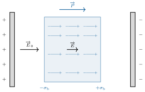
A dielectric is an insulator whose molecules acquire (or already own) electric dipole moments. The material’s response is summarised by the polarisation $\vect P$ : the dipole moment per unit volume, $\vect P = n\langle\vect p\rangle$ for $n$ molecules per unit volume. A polarised block carries bound charges — not free to leave, but perfectly real: a surface density $\sigma_{\text{b}} = \vect P\cdot\vect n$ where the polarisation meets the surface, and a volume density $\rho_{\text{b}} = -\nabla\cdot\vect P$ wherever it is non-uniform. A uniformly polarised slab is exactly equivalent to two sheets of charge $\pm P$ on its faces: all its interior dipole heads and tails cancel.

Proposition 22.2 (The displacement field)

Total charge is free plus bound; Gauss’s law with $\rho = \rho_{\text{f}} + \rho_{\text{b}}$ rearranges into a law for the electric displacement $\vect D = \varepsilon_0\vect E + \vect P$ :

\nabla\cdot\vect D = \rho_{\text{f}} :

$\vect D$ ’s sources are the free charges only — the ones on our plates and wires. In a linear dielectric the response is proportional, $\vect P = \varepsilon_0\chi_{\text{e}}\vect E$ , so $\vect D = \varepsilon_0\varepsilon_{\text{r}}\vect E$ with $\varepsilon_{\text{r}} = 1 + \chi_{\text{e}}$ the relative permittivity: air $1.0006$ , polyethylene $2.3$ , glass $\sim 5$ , water an enormous $80$ . Between capacitor plates held at fixed charge, $\vect D$ is unchanged by the dielectric, so $\vect E = \vect D/\varepsilon_0\varepsilon_{\text{r}}$ drops by $\varepsilon_{\text{r}}$ : the bound surface charges face the free ones and cancel most of their field. Capacitance is multiplied by $\varepsilon_{\text{r}}$ — the entire capacitor industry in one Greek letter.

Proof. $\nabla\cdot(\varepsilon_0\vect E) = \rho_{\text{f}} + \rho_{\text{b}} = \rho_{\text{f}} - \nabla\cdot\vect P$ ; move the polarisation term to the left. ∎

A dielectric slab between charged plates. The field aligns molecular dipoles; their interior charges cancel pairwise, leaving bound sheets _ b on the faces — which oppose the free charge and shrink the interior field from E_0 to E = E_0/ _ r. — A dielectric slab between charged plates. The field aligns molecular dipoles; their interior charges cancel pairwise, leaving bound sheets $\mp\sigma_{\text{b}}$ on the faces — which oppose the free charge and shrink the interior field from $\vect E_0$ to $\vect E = \vect E_0/\varepsilon_{\text{r}}$ .

22.2 Where permittivity comes from

Proposition 22.3 (Induced polarisation and Clausius–Mossotti)

An atom in a field $\vect E_{\text{loc}}$ stretches into a dipole $\vect p = \alpha\vect E_{\text{loc}}$ , with $\alpha$ the polarisability (dimension: $\varepsilon_0\times$ volume — roughly $\varepsilon_0$ times the atomic volume). In a dilute gas $E_{\text{loc}} \approx E$ and $\chi_{\text{e}} = n\alpha/\varepsilon_0$ is small. In a dense medium each molecule also feels its polarised neighbours: carving a small spherical cavity around it gives $\vect E_{\text{loc}} = \vect E + \vect P/3\varepsilon_0$ , and self-consistency yields the Clausius–Mossotti relation

\frac{\varepsilon_{\text{r}} - 1}{\varepsilon_{\text{r}} + 2} = \frac{n\alpha}{3\varepsilon_0} :

measure a vapour’s tiny susceptibility and predict the liquid’s — it works to a few percent for nonpolar liquids.

Proof. Admitted at this level. ∎

Remark 22.4

The cavity field $\vect P/3\varepsilon_0$ is the uniformly-polarised- sphere result quoted here without proof; the honest boundary-value derivation belongs to a dedicated electrodynamics course. Everything else above is bookkeeping.

Proposition 22.5 (Polar molecules: the Langevin function)

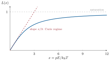
A molecule with a permanent dipole $p$ (water: $p = 6.2 \times 10^{-30}\,\mathrm{C}\,\mathrm{m}$ ) needs no stretching — only aligning, against thermal agitation. The canonical average of Chapter 17 over orientations, with energy $-pE\cos\theta$ , gives

\langle\cos\theta\rangle = L(x) = \coth x - \frac1x , \qquad x = \frac{pE}{k_{\text{B}}T} ,

the Langevin function: linear ( $L \approx x/3$ ) at small $x$ , saturating at $1$ when the field wins outright. In the linear regime $\chi_{\text{e}} = np^2/3\varepsilon_0k_{\text{B}}T$ — an electric Curie law, falling as $1/T$ : heat a polar liquid and its permittivity drops, the signature that distinguishes permanent from induced dipoles. For water at room temperature this predicts $\chi_{\text{e}} \sim 12$ — the right magnitude, with hydrogen-bond cooperation pushing the real value to $80$ .

Partial proof. $Z = \int_0^\pi \eu^{x\cos\theta}\,2\pi\sin\theta\,\dd\theta \propto \sinh x/x$ , and $\langle\cos\theta\rangle = \dd\ln Z/\dd x = \coth x - 1/x$ . Expanding $\coth x = 1/x + x/3 - \dots$ for small $x$ gives $L \approx x/3$ , hence $P = np\langle\cos\theta\rangle = np^2E/3k_{\text{B}}T$ . ∎

The Langevin function. Ordinary fields live far down in the linear regime (x 10-3 even at breakdown fields): full alignment of water’s dipoles would need E 7 × 108\, V/ m. — The Langevin function. Ordinary fields live far down in the linear regime ( $x \sim 10^{-3}$ even at breakdown fields): full alignment of water’s dipoles would need $E \sim 7 \times 10^{8}\,\mathrm{V}/\mathrm{m}$ .

22.3 Magnetisation and the field $H$

Definition 22.6 (Magnetisation, bound currents, and H)

The magnetic story runs in parallel. Matter is full of microscopic current loops — orbiting and spinning electrons, each a magnetic dipole $\vect\mu$ ; their density is the magnetisation $\vect M = n\langle\vect\mu\rangle$ . A uniformly magnetised block is equivalent to a bound surface current circulating around its sides (interior loops cancel pairwise; a bar magnet is a solenoid of bound current). Splitting currents into free and bound, Ampère’s law rearranges around the auxiliary field

\vect H = \frac{\vect B}{\mu_0} - \vect M , \qquad \oint \vect H\cdot\dd\vect\ell = I_{\text{free}} :

$\vect H$ is sourced by the currents in our wires (units $\mathrm{A}/\mathrm{m}$ ), while $\vect B$ keeps the physics — forces, flux, induction. Linear media have $\vect M = \chi_{\text{m}}\vect H$ and $\vect B = \mu_0(1 + \chi_{\text{m}})\vect H = \mu_0\mu_{\text{r}}\vect H$ .

Remark 22.7 (Three magnetic personalities)

Materials answer $\vect H$ in three ways. Diamagnets ( $\chi_{\text{m}} \sim -10^{-5}$ : water, copper, graphite) respond like Lenz’s law made permanent: the applied field perturbs every electron orbit so as to oppose it — weak, universal, temperature-independent, and repelled by magnets (a frog has been levitated this way in a $16\,\mathrm{T}$ bore). Paramagnets ( $\chi_{\text{m}} \sim +10^{-5}$ to $10^{-3}$ : aluminium, O $_2$ ) own permanent moments — unpaired spins from Chapter 14 — that align like Langevin’s dipoles: $\chi_{\text{m}} = \mu_0 n\mu^2/3k_{\text{B}}T$ , a Curie $1/T$ law (the quantum two-level version is Exercise 17.11). Ferromagnets (iron, cobalt, nickel: $\mu_{\text{r}}$ in the thousands) are paramagnets whose spins also talk to each other — the exchange coupling of Exercise 14.12 — and below the Curie temperature they align spontaneously: Theorem 21.4, now put to work.

22.4 Ferromagnetism at work: domains and hysteresis

Definition 22.8 (Domains and hysteresis)

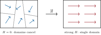
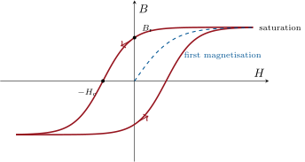
A raw lump of iron is not magnetised: it shatters into domains, micron-scale regions each fully magnetised but pointing differently, so the exterior field (and its energy cost) nearly cancels. An applied $\vect H$ moves the domain walls — favourable domains grow — and then rotates whole domains into line. Walls snag on defects, so the process is irreversible: sweep $H$ up and down and $B(H)$ traces a loop, the hysteresis cycle. Switch the current off and a remanent field $B_{\text{r}}$ survives; cancelling it needs the reverse coercive field $H_{\text{c}}$ . The loop’s enclosed area is energy dissipated per cycle and per unit volume. Soft materials (silicon steel, ferrites: thin loop, small $H_{\text{c}}$ ) make transformer and motor cores; hard ones (alnico, Nd $_2$ Fe $_{14}$ B: fat loop, huge $H_{\text{c}}$ ) make permanent magnets — and magnetic memory: the refrigerator magnet and the hard disk are hysteresis loops that refuse to forget.

Domains. Left: a virgin ferromagnet hides its magnetisation in mutually cancelling regions. Right: the applied field grows and rotates them into a single magnetised block — through irreversible wall jumps that give iron its memory.

The hysteresis cycle. From the virgin state (dashed), the field drives B to saturation; returning H to zero leaves the remanence B_ r, and only the coercive field -H_ c erases it. Loop area = heat per cycle per unit volume: thin loops for transformers, fat loops for permanent magnets. — The hysteresis cycle. From the virgin state (dashed), the field drives $B$ to saturation; returning $H$ to zero leaves the remanence $B_{\text{r}}$ , and only the coercive field $-H_{\text{c}}$ erases it. Loop area = heat per cycle per unit volume: thin loops for transformers, fat loops for permanent magnets.

Example 22.9 (The iron-core electromagnet)

Wind $N$ turns carrying $I$ around an iron ring ( $\mu_{\text{r}} \sim 5000$ ) with a small air gap $e$ . Ampère’s law for $\vect H$ around the loop: $H_{\text{iron}}\ell + H_{\text{gap}}e = NI$ , and flux continuity makes $B$ common, so

B\Big(\frac{\ell}{\mu_0\mu_{\text{r}}} + \frac{e}{\mu_0}\Big) = NI .

With $\ell = 1\,\mathrm{m}$ and $e = 1\,\mathrm{cm}$ , the gap term is fifty times the iron term: nearly all the coil’s effort is spent pushing field across one centimetre of air. That is the magnetic circuit in one line — iron is a near-perfect conductor of flux, air the resistor — and it is why motors, relays and scrapyard lifters keep their air gaps ruthlessly thin (Problem 22.1).

A ferrofluid over a hidden magnet: the liquid’s magnetisation makes field energy cheaper than gravity and surface tension, and the surface buckles into a lattice of spikes — M, made visible. — A ferrofluid over a hidden magnet: the liquid’s magnetisation makes field energy cheaper than gravity and surface tension, and the surface buckles into a lattice of spikes — $\vect M$ , made visible.

22.5 Exercises

Exercise 22.1 ★

Bound-charge bookkeeping. A slab of thickness $d$ is uniformly polarised along its normal, magnitude $P$ . (a) Give the bound charge densities on each face. (b) Show the field inside due to those sheets is $E = P/\varepsilon_0$ , opposing $\vect P$ . (c) What is $\vect D$ inside, with no free charge anywhere? (d) A bar electret (frozen-in $\vect P$ ) is the electric analogue of which magnetic object?

Solution

Solution of Exercise 22.1.

(a) $+P$ on the face $\vect P$ points at, $-P$ on the other. (b) Two infinite sheets $\pm P$ produce $P/\varepsilon_0$ between them, directed from $+$ to $-$ , i.e. against $\vect P$ . (c) $\vect D = \varepsilon_0\vect E + \vect P = 0$ — as it must be: no free charge, and $\vect D$ ’s normal component is continuous from the vacuum outside. (d) A bar magnet: frozen-in dipole density, field sustained by its own bound sources.

Exercise 22.2 ★

Capacitor with dielectric. A parallel-plate capacitor ( $C_0 = 100\,\mathrm{pF}$ ) is charged to $12\,\mathrm{V}$ and disconnected. A slab with $\varepsilon_{\text{r}} = 4$ fills it. Find (a) the new capacitance; (b) the new voltage; (c) the energy before and after — where did the difference go? (d) Repeat (b)–(c) with the battery kept connected.

Solution

Solution of Exercise 22.2.

(a) $C = \varepsilon_{\text{r}}C_0 = 400\,\mathrm{pF}$ . (b) $Q = 1.2\,\mathrm{nC}$ is trapped: $V = Q/C = 3\,\mathrm{V}$ . (c) $\tfrac12C_0V_0^2 = 7.2\,\mathrm{nJ}$ before, $1.8\,\mathrm{nJ}$ after: the missing $5.4\,\mathrm{nJ}$ became mechanical work — the fringing field pulls the slab in. (d) Battery connected: $V$ stays $12\,\mathrm{V}$ , $Q$ quadruples, energy rises to $28.8\,\mathrm{nJ}$ — the battery pays for both the new field energy and the pull.

Exercise 22.3 ★

The susceptibility zoo. Classify (dia-, para-, or ferromagnetic) and justify from electronic structure where you can: water ( $\chi_{\text{m}} = -9\times10^{-6}$ ), aluminium ( $+2.2\times10^{-5}$ ), liquid oxygen ( $+3.5\times10^{-3}$ — why is O $_2$ magnetic at all?), nickel ( $\mu_{\text{r}} \sim 600$ at small field). Which of the four would a strong magnet visibly attract, and which ever so slightly repel?

Solution

Solution of Exercise 22.3.

Water: diamagnetic — all electrons paired, only Larmor-induced opposition. Aluminium: paramagnetic (conduction electrons’ spins). Liquid oxygen: strongly paramagnetic — O $_2$ carries two unpaired electrons (Hund’s rule filling of its antibonding orbitals, Chapter 14); it visibly sticks between magnet poles. Nickel: ferromagnetic. The magnet visibly attracts nickel and liquid oxygen, and ever-so-slightly repels water — the dimple a strong magnet makes in a water surface.

Exercise 22.4 ★

$B$ , $H$ , $M$ . A long solenoid ( $n = 2000$ turns per metre, $I = 1.5\,\mathrm{A}$ ) is filled with iron, and $B = 1.6\,\mathrm{T}$ is measured. Compute (a) $H$ ; (b) $M$ ; (c) the amplification $B/\mu_0H$ ; (d) the bound surface current per metre equivalent to $M$ — compare it with the coil’s own $nI$ .

Solution

Solution of Exercise 22.4.

(a) $H = nI = 3000\,\mathrm{A}/\mathrm{m}$ . (b) $M = B/\mu_0 - H = 1.27 \times 10^{6}\,\mathrm{A}/\mathrm{m}$ . (c) $B/\mu_0H \approx 420$ . (d) The equivalent bound sheet current is $M \approx 1.27 \times 10^{6}\,\mathrm{A}$ per metre — four hundred times the coil’s own $nI = 3000\,\mathrm{A}/\mathrm{m}$ : the iron is doing almost all the work.

Exercise 22.5 ★★

Coaxial cable, insulated. A coaxial line (inner radius $a$ , outer $b$ ) carries free charge $\lambda$ per unit length on the core, with dielectric $\varepsilon_{\text{r}}$ between. (a) Find $\vect D(r)$ from symmetry. (b) Deduce $\vect E$ and $\vect P$ . (c) Compute the bound charge densities at $r = a$ and $r = b$ and check they sum to zero per unit length. (d) Show the capacitance per unit length is multiplied by $\varepsilon_{\text{r}}$ .

Solution

Solution of Exercise 22.5.

(a) A cylindrical Gauss surface encloses only free charge: $D = \lambda/2\pi r$ , radial. (b) $E = \lambda/2\pi\varepsilon_0\varepsilon_{\text{r}}r$ , $P = (\varepsilon_{\text{r}}-1)\lambda/2\pi\varepsilon_{\text{r}}r$ . (c) $\sigma_{\text{b}}(a) = -P(a)$ : per unit length $-(\varepsilon_{\text{r}}-1)\lambda/\varepsilon_{\text{r}}$ ; at $r = b$ , $+P(b)$ : per unit length $+(\varepsilon_{\text{r}}-1)\lambda/\varepsilon_{\text{r}}$ — sum zero, as bound charge must. (d) $V = \int E\,\dd r = (\lambda/2\pi\varepsilon_0\varepsilon_{\text{r}})\ln(b/a)$ , so $C/\ell = 2\pi\varepsilon_0\varepsilon_{\text{r}}/\ln(b/a)$ : multiplied by $\varepsilon_{\text{r}}$ .

Exercise 22.6 ★★

Clausius–Mossotti at work. Gaseous argon at $1\,\mathrm{bar}$ , $300\,\mathrm{K}$ has $\varepsilon_{\text{r}} = 1.00052$ . (a) Extract $\alpha/\varepsilon_0$ (a volume) and compare with the atomic volume. (b) Liquid argon has $n = 2.1 \times 10^{28}\,\mathrm{m}^{-3}$ : predict $\varepsilon_{\text{r}}$ from Clausius–Mossotti (measured: 1.53). (c) Why does the naive $\chi = n\alpha/\varepsilon_0$ overshoot less badly here than for water? (d) For which molecules must the whole scheme fail, and what replaces it?

Solution

Solution of Exercise 22.6.

(a) $n = P/k_{\text{B}}T = 2.4 \times 10^{25}\,\mathrm{m}^{-3}$ , so $\alpha/\varepsilon_0 = \chi/n \approx 2.2 \times 10^{-29}\,\mathrm{m}^{3}$ — the volume of a sphere of radius $\approx1.7\,\text{Å}$ : polarisability is atomic volume, in $\varepsilon_0$ units. (b) $n\alpha/3\varepsilon_0 = 0.15$ , so $(\varepsilon_{\text{r}} - 1)/(\varepsilon_{\text{r}} + 2) = 0.15$ gives $\varepsilon_{\text{r}} = 1.53$ — dead on the measured value. (c) The local-field correction is a 15 % effect here; argon is nonpolar, so there is no orientation contribution to run away. (d) Polar molecules (water, HCl): permanent dipoles dominate and interact; Langevin–Debye (and, for dense liquids, Onsager) theory replaces the simple cavity argument.

Exercise 22.7 ★★

Water’s giant permittivity. (a) From Proposition 22.5, compute $\chi_{\text{e}} = np^2/3\varepsilon_0k_{\text{B}}T$ for water ( $n = 3.3 \times 10^{28}\,\mathrm{m}^{-3}$ , $p = 6.2 \times 10^{-30}\,\mathrm{C}\,\mathrm{m}$ , $T = 300\,\mathrm{K}$ ). (b) Estimate the field needed for $x = 1$ (serious saturation) and compare with water’s dielectric strength $\sim7 \times 10^{7}\,\mathrm{V}/\mathrm{m}$ . (c) Microwave ovens run at $2.45\,\mathrm{GHz}$ : why does a lossy rotating-dipole response heat food, and why does ice heat far more slowly than liquid water? (d) Predict the sign of $\dd\varepsilon_{\text{r}}/\dd T$ for water and for argon.

Solution

Solution of Exercise 22.7.

(a) $\chi_{\text{e}} = np^2/3\varepsilon_0k_{\text{B}}T \approx 11.5$ . (b) $E = k_{\text{B}}T/p \approx 6.7 \times 10^{8}\,\mathrm{V}/\mathrm{m}$ — ten times the breakdown field: water always operates deep in the linear regime. (c) At $2.45\,\mathrm{GHz}$ the dipoles almost keep up but lag: the out-of-phase part of the response does net work on the water every cycle — dielectric heating. In ice the molecules are locked to the lattice; their rotational relaxation sits at kilohertz, so at gigahertz ice barely absorbs (defrost cycles pulse gently, letting melted water do the heating). (d) Water: negative ( $1/T$ orientation response); argon: essentially zero — induced polarisability does not care about temperature.

Exercise 22.8 ★★

Diamagnetism estimated. Treat an atomic electron as a charge on a ring of radius $r$ ; an applied $B$ changes its angular frequency by the Larmor shift $\Delta\omega = eB/2m_{\text{e}}$ . (a) Show the induced moment is $\Delta\mu = -e^2r^2B/4m_{\text{e}}$ (opposing $B$ ). (b) Averaging orientations and summing $Z$ electrons per atom, one finds $\chi_{\text{m}} = -\mu_0ne^2Z\langle r^2\rangle/6m_{\text{e}}$ : evaluate for water ( $n = 3.3 \times 10^{28}\,\mathrm{m}^{-3}$ molecules, $Z = 10$ , $\langle r^2\rangle \approx (0.7\,\text{Å})^2$ ) and compare with the measured $-9\times10^{-6}$ . (c) Why is diamagnetism temperature-independent while paramagnetism is not? (d) Why does even a frog levitate in $16\,\mathrm{T}$ , and why must the magnet’s field be non-uniform?

Solution

Solution of Exercise 22.8.

(a) The Larmor shift changes the circulating current by $\Delta I = -e\Delta\omega/2\pi = -e^2B/4\pi m_{\text{e}}$ , hence $\Delta\mu = \Delta I\cdot\pi r^2 = -e^2r^2B/4m_{\text{e}}$ , opposing $\vect B$ whichever way the electron orbits — Lenz’s law at the atomic scale. (b) With the stated numbers, $\chi_{\text{m}} \approx -9.5\times10^{-6}$ : the measured $-9\times10^{-6}$ , from a ring model. (c) The induced moment comes from orbit distortion, not from a Boltzmann competition between alignment and disorder — no $T$ anywhere. (d) Water is diamagnetic, so the frog is pushed toward weak field; the force density $\propto \chi\,\nabla(B^2/2\mu_0)$ vanishes in a uniform field — levitation needs $B\,\dd B/\dd z$ large enough to balance $\rho g$ , hence the $16\,\mathrm{T}$ bore.

Exercise 22.9 ★★

Curie paramagnetism and cooling. A salt carries $n = 2 \times 10^{27}\,\mathrm{m}^{-3}$ ions of moment $\mu \approx \mu_{\text{B}}$ . (a) Compute $\chi_{\text{m}} = \mu_0n\mu^2/3k_{\text{B}}T$ at $300\,\mathrm{K}$ and at $1\,\mathrm{K}$ . (b) At what temperature would $\chi_{\text{m}}$ reach $1$ — and what physics (neglected here) intervenes first in most salts? (c) Adiabatic demagnetisation: magnetise at $1\,\mathrm{K}$ , isolate, then remove the field slowly — explain with the spin entropy of Chapter 16 why the sample cools. (d) Why does the method need a paramagnet rather than a ferromagnet?

Solution

Solution of Exercise 22.9.

(a) $\chi_{\text{m}} = \mu_0n\mu_{\text{B}}^2/3k_{\text{B}}T \approx 1.7\times10^{-5}$ at $300\,\mathrm{K}$ , $5\times10^{-3}$ at $1\,\mathrm{K}$ . (b) Extrapolating, $\chi \to 1$ near $5\,\mathrm{mK}$ — but dipolar and exchange couplings order (or freeze) real salts first: Curie’s law is a high-temperature law. (c) Magnetised at $1\,\mathrm{K}$ , the spin entropy is squeezed out into the bath; isolated, $S$ is fixed, and lowering $B$ lets the spins reclaim their $k_{\text{B}}\ln 2$ each — the energy comes from the lattice, whose temperature falls (millikelvins in practice). (d) A ferromagnet’s spins order themselves below $T_{\text{c}}$ : their entropy is no longer field-controlled, and hysteresis would dissipate instead of cool.

Exercise 22.10 ★★★

The magnetic circuit. An iron torus ( $\ell = 60\,\mathrm{cm}$ , $\mu_{\text{r}} = 4000$ , section $A = 16\,\mathrm{cm}^{2}$ ) carries $N = 500$ turns and a gap $e = 4\,\mathrm{mm}$ . (a) Show $NI = B(\ell/\mu_0\mu_{\text{r}} + e/\mu_0)$ and compute the current for $B = 1.2\,\mathrm{T}$ . (b) What fraction of $NI$ is spent on the gap? (c) Define the reluctance $\mathcal R = \ell/\mu A$ of each segment and restate (a) as a series “Ohm’s law” for flux. (d) The iron saturates near $1.8\,\mathrm{T}$ : explain what happens to the circuit model — and to your motor — beyond it.

Solution

Solution of Exercise 22.10.

(a) $NI = B(\ell/\mu_0\mu_{\text{r}} + e/\mu_0)$ : with $\ell/\mu_{\text{r}} = 0.15\,\mathrm{mm}$ -equivalent versus $e = 4\,\mathrm{mm}$ , $NI \approx 3960$ ampere-turns, $I \approx 7.9\,\mathrm{A}$ . (b) $4/4.15 \approx 96\,\%$ of the effort crosses the gap. (c) $\Phi = NI/(\mathcal R_{\text{iron}} + \mathcal R_{\text{gap}})$ with $\mathcal R = \ell/\mu A$ : magnetomotive force $NI$ plays voltage, flux plays current, reluctance plays resistance — here $\mathcal R_{\text{gap}} \approx 2.0\times10^{6}\,\mathrm{H}^{-1} \approx 27\,\mathcal R_{\text{iron}}$ . (d) Past $1.8\,\mathrm{T}$ the iron’s incremental $\mu_{\text{r}}$ collapses toward 1: its reluctance soars, extra current buys almost no extra flux, and a motor pushed there stops gaining torque while its windings cook.

Exercise 22.11 ★★★

Hysteresis losses. A transformer core (volume $4 \times 10^{-3}\,\mathrm{m}^{3}$ ) runs at $50\,\mathrm{Hz}$ . Its silicon-steel loop encloses $\sim40\,\mathrm{J}/\mathrm{m}^{3}$ per cycle. (a) Compute the hysteresis power loss. (b) The same core in hard steel ( $\sim6 \times 10^{3}\,\mathrm{J}/\mathrm{m}^{3}$ ): loss, and verdict. (c) Eddy currents add a loss $\propto f^2$ : explain why cores are laminated and why ferrites take over at radio frequencies. (d) A hard disk bit must keep its magnetisation against thermal kicks for ten years: relate the demands on $H_{\text{c}}$ for memory to those for a transformer, and conclude that no single material can do both jobs.

Solution

Solution of Exercise 22.11.

(a) $P = wfV = 40\times50\times4 \times 10^{-3} = 8\,\mathrm{W}$ — acceptable. (b) $1.2\,\mathrm{kW}$ : the core would glow; hard steel is disqualified from AC service by its own virtue. (c) Eddy EMFs scale with loop area and $f$ ; laminating (or powdering, or using insulating ferrites) chops the loops, cutting the $f^2$ loss — which is why ferrites own the megahertz range. (d) Memory wants the stored bit’s barrier $\sim\mu_0H_{\text{c}}M_{\text{s}}V \gg k_{\text{B}}T$ for a decade (the superparamagnetic limit), i.e. $H_{\text{c}}$ as large as writable; a transformer wants $H_{\text{c}} \to 0$ for a thin loop. One material cannot sit at both ends: soft magnets for machines, hard magnets for memory.

Exercise 22.12 ★★★

The demagnetising field. Inside a uniformly magnetised body with no free current, $\oint\vect H\cdot\dd\vect\ell = 0$ forces $\vect H$ inside to oppose $\vect M$ ( $\vect H = -N_{\text{d}}\vect M$ , with $N_{\text{d}}$ a shape factor: $1/3$ for a sphere, $\approx 0$ along a long needle, $\approx 1$ across a thin plate). (a) Justify the needle and plate limits with the bound-current (solenoid) picture. (b) Why does a stubby magnet partially demagnetise itself while a needle keeps its magnetisation? (c) Connect to compass needles and to the elongated grains of magnetic tape. (d) A soft-iron sphere sits in a uniform external $B_0$ : explain why its response saturates at $\vect H \approx 0$ inside, i.e. $M \approx 3B_0/\mu_0$ at most, however large $\mu_{\text{r}}$ is.

Solution

Solution of Exercise 22.12.

(a) A long axially magnetised needle is a long solenoid of bound current: inside, $H \approx 0$ (all $B$ comes from $M$ ). A thin plate magnetised across its faces is the shortest, fattest solenoid possible: its interior return field gives $H = -M$ . (b) The stubby magnet works at $H = -N_{\text{d}}M$ , well down its demagnetisation curve: wall motion nibbles the remanence away; a needle sits at $H \approx 0$ and keeps what it has. (c) Hence compass needles, and the elongated single-domain grains of magnetic tape and early hard disks — shape anisotropy as memory insurance. (d) Flux conservation and $\oint\vect H\cdot \dd\vect\ell = 0$ give the interior of a sphere $H_{\text{in}} = H_0 - M/3$ ; as $\mu_{\text{r}}\to\infty$ the iron drives $H_{\text{in}}\to0$ , so $M \to 3H_0 = 3B_0/\mu_0$ : the sphere can concentrate the field only threefold, however “good” the iron.

The weekend problem, at work: an iron-cored coil whose field magnetises the scrap itself — and lets go on command, which is the half of the design that hysteresis makes interesting.

22.6 Problem: The scrapyard lifter

Problem 22.1

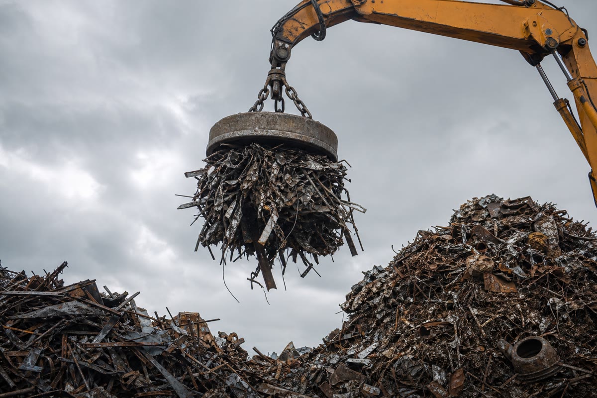
The scrapyard lifter. A recycling yard orders a crane electromagnet: a flat-faced iron pot, one metre across, that must lift crushed-car bales of two tonnes, then — just as important — drop them on command. You are the design engineer.

Part I — Why iron.

The bare coil: 400 turns carrying $25\,\mathrm{A}$ spread over a magnetic path of $\sim1\,\mathrm{m}$ . Estimate $B \sim \mu_0NI/\ell$ with no iron.
Explain in two sentences, with domains, why filling the coil with iron multiplies this by $\sim\mu_{\text{r}}$ .
Iron’s magnetisation saturates at $M_{\text{s}} \approx 1.7 \times 10^{6}\,\mathrm{A}/\mathrm{m}$ . Compute the ceiling $\mu_0M_{\text{s}}$ this puts on the pole field, whatever the coil does.
Each iron atom contributes $\approx 2.2$ Bohr magnetons. Check: with $n = 8.5 \times 10^{28}\,\mathrm{m}^{-3}$ , recover $M_{\text{s}}$ .
Why must the pole faces be machined flat and kept free of rust and grit? (Think of Example 22.9.)
The load itself becomes part of the magnetic circuit. Sketch the flux path: pot core, north face, steel bale, south face, back through the yoke.

Part II — The magnetic circuit and the force.

Model the circuit: iron path $\ell = 1.2\,\mathrm{m}$ , $\mu_{\text{r}} = 2000$ , and two effective air gaps (face–bale contact) of $e = 1.5\,\mathrm{mm}$ each. Write Ampère’s law for $H$ around the loop.
Compute the three reluctance terms per unit area ( $\ell/\mu_{\text{r}}$ versus $2e$ ) and show the millimetre gaps still consume most of the coil’s effort.
With $NI = 10\,000$ ampere-turns, compute $B$ in the gaps.
The lifting pressure on each pole face is $B^2/2\mu_0$ (magnetic energy density released per metre of approach). Evaluate it in $\mathrm{kPa}$ for your $B$ .
Total pole-face area $A = 0.12\,\mathrm{m}^{2}$ : compute the lifting force and convert to tonnes.
Does it meet the two-tonne specification with a factor-two margin? If not, adjust $NI$ and state the new current.
Crushed bales touch the faces on perhaps a third of their area, with wider effective gaps. Recompute the force for $e = 4\,\mathrm{mm}$ , $A_{\text{eff}} = 0.04\,\mathrm{m}^{2}$ and comment on why rated lifts quote “flat plate” capacity.

Part III — Remembering and forgetting.

The yard flips the switch to drop a bale — and it hangs on. Name the culprit, with the hysteresis loop.
Why must the pot be soft iron (small $H_{\text{c}}$ , small $B_{\text{r}}$ ) rather than hard magnet steel?
Even soft iron keeps a little remanence. Propose the standard cure: a brief reversed current pulse — which point of the loop is it aiming for?
Some controllers instead apply a decaying alternating current. Sketch what the $B$ – $H$ trajectory does and why it ends demagnetised.
The crane also handles hot slabs straight from a furnace, at $800\,{}^{\circ}\mathrm{C}$ . Iron’s Curie point is $1043\,\mathrm{K}$ : what happens to the lift force, and why? (Theorem 21.4.)
A summer apprentice suggests saving copper by doubling the gap and doubling $NI$ . Use your Part II formulas to explain the asymmetry: which halves and which merely holds?

Part IV — Power, heat, and the bill.

The coil: 400 turns of copper, mean turn length $2.5\,\mathrm{m}$ , wire section $16\,\mathrm{mm}^{2}$ , resistivity $\rho = 1.7 \times 10^{-8}\,\Omega\,\mathrm{m}$ . Compute its resistance.
At $I = 25\,\mathrm{A}$ : the dissipated power, and the daily energy for an eight-hour shift at $60\,\%$ duty.
The magnetic energy stored in the two gaps ( $B^2/2\mu_0 \times$ volume): compute it and compare with one second of coil dissipation. Where does all the rest of the electrical energy go?
Dropping the load returns almost none of the stored energy to the grid. Explain, with the loop area and the inductive spike, why the controller needs a freewheel (flyback) path across the coil.
Power fails with a bale in the air. What does the bale do, and what does the remanence alone hold? Justify the yard rule that nobody walks under a powered magnet — and the sales pitch for battery-backed lifters.
Sum up the design in four lines: field ceiling set by $M_{\text{s}}$ , force by $B^2A/2\mu_0$ , controllability by soft-iron hysteresis, operating cost by $RI^2$ — the whole chapter hanging from one crane.

Solution

Solution of Problem 22.1.

1. $B \approx \mu_0NI/\ell = 13\,\mathrm{mT}$ — a refrigerator-magnet field from $250\,\mathrm{W}$ of coil. 2. The coil’s small $H$ unpins and rotates domains whose bound currents then circulate in step with the coil’s: the iron adds $\mu_0M \gg \mu_0H$ of its own. 3. $\mu_0M_{\text{s}} = 2.1\,\mathrm{T}$ : no coil can pull more from iron’s poles. 4. $M = 2.2\mu_{\text{B}}n = 2.2\times9.27 \times 10^{-24} \times8.5 \times 10^{28} \approx 1.7 \times 10^{6}\,\mathrm{A}/\mathrm{m}$ — consistent. 5. Any rust or grit is an extra series air gap in the one place reluctance matters most; a tenth of a millimetre of scale measurably eats the force. 6. Flux leaves the central north pole, crosses the contact gap into the bale, runs through the steel, and returns through the outer annular south pole and the yoke — the load closes the magnetic circuit. 7. $NI = H_{\text{iron}}\ell + 2H_{\text{gap}}e = B(\ell/\mu_0\mu_{\text{r}} + 2e/\mu_0)$ . 8. Per unit area: $\ell/\mu_{\text{r}} = 0.6\,\mathrm{mm}$ versus $2e = 3\,\mathrm{mm}$ : the three millimetres of air take $\sim83\,\%$ of the ampere-turns. 9. The linear formula gives $B = \mu_0NI/(\ell/ \mu_{\text{r}} + 2e) \approx 3.5\,\mathrm{T}$ — above the question-3 ceiling: the pot saturates and delivers $B \approx 1.7\,\mathrm{T}$ , coil straining notwithstanding. 10. $B^2/2\mu_0 \approx 1.15 \times 10^{6}\,\mathrm{Pa} \approx 1150\,\mathrm{kPa}$ — eleven atmospheres of pull. 11. $F = 1.15 \times 10^{6}\times0.12 \approx 140\,\mathrm{kN} \approx 14$ tonnes. 12. Yes: 14 tonnes against a 4-tonne requirement (2 tonnes $\times$ safety factor 2) — the margin exists for question 13’s sake. 13. With $e = 4\,\mathrm{mm}$ and $A_{\text{eff}} = 0.04\,\mathrm{m}^{2}$ : $B \approx 1.5\,\mathrm{T}$ , pressure $\approx870\,\mathrm{kPa}$ , force $\approx35\,\mathrm{kN} \approx 3.5$ tonnes — the twelve-tonne “flat plate” rating shrinks to barely the spec on real scrap, which is why capacity is always quoted on ground plate. 14. Remanence: switch off and the iron sits at $B_{\text{r}}$ on its loop — the pot is now a weak permanent magnet, and light loads hang on. 15. Soft iron’s thin loop makes $B_{\text{r}}$ and $H_{\text{c}}$ small: the magnet must forget on command; hard steel would turn the lifter into a permanent magnet with a switch that does nothing. 16. A calibrated reverse pulse drives the material to $-H_{\text{c}}$ , the loop’s zero- $B$ crossing, and releases the load. 17. A decaying AC sweep traces ever-smaller nested loops spiralling into the origin: the demagnetised state — the same degaussing used on ship hulls and old CRT screens. 18. $800\,{}^{\circ}\mathrm{C}$ is $1073\,\mathrm{K}$ $> T_{\text{c}}$ : the slab is paramagnetic — $\mu_{\text{r}} \approx 1$ , the circuit opens, the force collapses; hot mills move slabs with tongs, not magnets. 19. Doubling $e$ halves $B$ and quarters the force (gap-dominated circuit); doubling $NI$ restores both — but $P = RI^2$ quadruples: gaps are paid for in copper heat. 20. $R = \rho L/A = 1.7 \times 10^{-8}\times1000/ 1.6 \times 10^{-5} \approx 1.1\,\Omega$ . 21. $P = RI^2 \approx 660\,\mathrm{W}$ ; over $8\,\text{h}\times0.6$ : $\approx3.2\,\mathrm{kWh}$ per shift — a few euros of electricity to move hundreds of tonnes. 22. Gap volume $2Ae = 3.6 \times 10^{-4}\,\mathrm{m}^{3}$ at $1.15 \times 10^{6}\,\mathrm{J}/\mathrm{m}^{3}$ : $\approx410\,\mathrm{J}$ — less than one second of coil heating. Steady-state, essentially all electrical input becomes copper heat; the field, once built, costs only its maintenance current. 23. Opening the circuit forces $LI$ to zero abruptly: the coil answers with a huge inductive spike that arcs the contacts; a freewheel diode (or resistor) lets the stored field energy die quietly as heat — and the loop’s area is dissipated in the iron each cycle regardless. 24. The lifting force needs current: the bale drops. Remanence retains only a token force — kilograms, not tonnes. Hence the walkway rule, and battery-backed (or permanent-magnet plus release-coil) lifters for anything that dangles over people. 25. Ceiling: $\mu_0M_{\text{s}} \approx 2\,\mathrm{T}$ . Force: $B^2A/2\mu_0$ , ruled by millimetres of air gap. Control: soft iron, small $B_{\text{r}}$ , degauss pulse to drop. Cost: $RI^2$ , a kilowatt-scale heater — the chapter, hanging from a crane.

Terms defined in this chapter

See all 431 terms in the glossary

22.1 Polarisation and the displacement field

22.2 Where permittivity comes from

22.3 Magnetisation and the field HHH

22.4 Ferromagnetism at work: domains and hysteresis

22.5 Exercises

22.6 Problem: The scrapyard lifter

Terms defined in this chapter

22.3 Magnetisation and the field $H$