University Physics — Year 3 · Bachelor Year 3

12Spin and Two-Level Systems

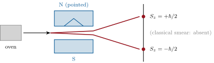
In 1922 Stern and Gerlach sent a beam of silver atoms through a lopsided magnet, expecting either no deflection or a continuous smear. The beam split cleanly in two. No orbital angular momentum can do that: $2l + 1$ is always odd. The atoms were announcing a new, purely quantum possession — spin, an intrinsic angular momentum of $j = \tfrac12$ , the half-integer rung the algebra of Chapter 10 kept ready and orbits could never use. Spin doubles every electron state (completing the count behind the periodic table), carries the magnetism of iron and of the proton, and is the cleanest two-level system nature offers: the physics of this chapter runs the magnetic resonance scanner in every hospital, the caesium clock that defines the second, the 21-centimetre whisper by which galaxies are mapped, and the qubit.

12.1 The experiment that found it

Example 12.1 (Stern–Gerlach)

A magnetic moment $\vect\mu$ in an inhomogeneous field feels the force $F_z = \mu_z\,\partial B_z/\partial z$ : the deflection measures $\mu_z$ . Classical expectation: moments oriented at random, a continuous fan. Quantum expectation for orbital momenta: $2l + 1$ spots: one, three, five — always odd. Observed for silver (and for hydrogen): two spots, symmetric, nothing between. The measured component takes exactly two values — the signature of $j = \tfrac12$ , forbidden to orbits, and the direct display of quantisation: the apparatus is a measuring device for one spin component, and the beam splits into its two eigenvalues.

The Stern–Gerlach experiment: an inhomogeneous field pulls opposite moments opposite ways, turning the magnet into a measuring apparatus for one spin component. Silver atoms land in two spots — a two-valued observable, caught in the act.

Definition 12.2 (Spin one-half)

The electron (and the proton, the neutron, the quarks) carries an intrinsic angular momentum with $j = \tfrac12$ : a two-dimensional state space spanned by $\ket\uparrow, \ket\downarrow$ (eigenstates of $\hat S_z$ with $\pm\hbar/2$ ), on which

\hat{\vect S} = \frac\hbar2\,\hat{\vect\sigma} , \qquad \sigma_x = \begin{pmatrix}0&1\\1&0\end{pmatrix} ,\; \sigma_y = \begin{pmatrix}0&-\iu\\\iu&0\end{pmatrix} ,\; \sigma_z = \begin{pmatrix}1&0\\0&-1\end{pmatrix}

— the Pauli matrices, realising the angular momentum algebra in its smallest possible home. A general state $\alpha\ket\uparrow + \beta\ket\downarrow$ is a spinor. The electron’s magnetic moment is

\hat{\vect\mu} = -g\,\frac{\mu_{\text{B}}}{\hbar}\,\hat{\vect S} , \qquad g \approx 2 :

twice the orbital rate per unit angular momentum — the anomaly Einstein–de Haas had measured (Exercise 10.12) and the Dirac equation would later predict. Spin is not a rotation of anything: no radius, no “spinning ball” survives scrutiny — it is intrinsic, like charge.

Example 12.3 (Chained Stern–Gerlach filters)

Select the $S_z = +\hbar/2$ beam, and measure $S_z$ again: all atoms answer $+$ . Measure $S_x$ instead: half and half — the state $\ket\uparrow$ is the superposition $(\ket{+x} + \ket{-x})/\sqrt2$ . Now keep the $S_x = +$ beam and measure $S_z$ once more: half and half again — the $S_x$ measurement erased the previously sharp $S_z$ . Three magnets suffice to exhibit incompatibility, collapse and Born’s rule; this chain is Example 8.7 performed with atoms.

12.2 The Bloch sphere

Proposition 12.4 (Spin along any axis)

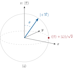
For the unit direction $\vect n = (\sin\theta\cos\varphi, \sin\theta\sin\varphi, \cos\theta)$ , the operator $\vect n\cdot\hat{\vect\sigma}$ has eigenvalues $\pm1$ , with

\ket{+\vect n} = \cos\tfrac\theta2\,\ket\uparrow + \eu^{\iu\varphi}\sin\tfrac\theta2\,\ket\downarrow .

Every pure spinor is $\ket{+\vect n}$ for exactly one direction: the state space maps onto a sphere — the Bloch sphere — with orthogonal states at antipodes (note the half-angles: opposite directions, not perpendicular ones, are orthogonal). Rotations of the sphere are exactly the evolutions a magnetic field generates: the geometry of every qubit manipulation ever performed.

Partial proof. Diagonalise the $2\times2$ matrix $\vect n\cdot\vect\sigma = \begin{pmatrix}\cos\theta & \sin\theta\,\eu^{-\iu\varphi}\\ \sin\theta\,\eu^{\iu\varphi} & -\cos\theta\end{pmatrix}$ : trace $0$ , determinant $-1$ , eigenvalues $\pm1$ ; the given spinor is checked by substitution (half-angle identities). Antipodes: $\theta \to \pi - \theta$ , $\varphi \to \varphi + \pi$ gives $\braket{+\vect n'}{+\vect n} = 0$ . ∎

The Bloch sphere: every spin-1/2 state is a point; poles are ,, the equator holds their equal superpositions, and orthogonal states sit at antipodes. Magnetic fields rotate the sphere — the control panel of the qubit. — The Bloch sphere: every spin- $\tfrac12$ state is a point; poles are $\ket\uparrow, \ket\downarrow$ , the equator holds their equal superpositions, and orthogonal states sit at antipodes. Magnetic fields rotate the sphere — the control panel of the qubit.

12.3 Spin in a field: precession and resonance

Proposition 12.5 (Larmor precession)

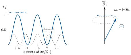
In a static field $\vect B_0 = B_0\vect e_z$ , the Hamiltonian $\hat H = -\hat{\vect\mu}\cdot\vect B_0$ splits the two levels by $\hbar\omega_0$ and makes the mean spin precess about the field:

\frac{\dd\langle\hat{\vect S}\rangle}{\dd t} = \gamma\,\langle\hat{\vect S}\rangle\wedge\vect B_0 , \qquad \omega_0 = |\gamma|B_0 ,

with the gyromagnetic ratio $\gamma$ ( $\mu = \gamma S$ ). The Bloch vector turns about $z$ at $\omega_0$ , its angle to the field frozen — exactly the classical gyroscope picture, exact here because the commutators are linear. For the electron: $28\,\mathrm{GHz}/\mathrm{T}$ ; for the proton (moment $2.79$ nuclear magnetons): $\gamma_p/2\pi = 42.6\,\mathrm{MHz}/\mathrm{T}$ — the licence plate of every MRI machine.

Proof. Apply Proposition 8.12 with $\hat H = -\gamma B_0\hat S_z$ : the commutators give $\dd\langle\hat S_x\rangle/\dd t = -\gamma B_0\langle\hat S_y\rangle$ , $\dd\langle\hat S_y\rangle/\dd t = +\gamma B_0\langle\hat S_x\rangle$ and $\dd\langle\hat S_z\rangle/\dd t = 0$ , which assemble into the stated vector product. ∎

Proposition 12.6 (Magnetic resonance)

Add a small field $B_1$ rotating in the transverse plane at frequency $\omega$ . In the frame rotating with it, $B_0$ is effectively reduced to $(\omega_0 - \omega)/|\gamma|$ ; at resonance ( $\omega = \omega_0$ ) only $B_1$ survives, and the spin precesses about it at the Rabi frequency $\Omega_1 = |\gamma|B_1$ : starting from $\ket\uparrow$ , the probability of having flipped is

\mathcal P_\downarrow(t) = \sin^2\Big(\frac{\Omega_1t}{2}\Big) .

A pulse of duration $\pi/\Omega_1$ (a “ $\pi$ pulse”) inverts the spin; half of it (a “ $\pi/2$ pulse”) lays it in the equatorial plane, where it precesses at $\omega_0$ and, by Faraday induction, broadcasts its frequency into any nearby coil. Off resonance the flopping amplitude collapses as $\Omega_1^2/[\Omega_1^2 + (\omega - \omega_0)^2]$ : the response is sharply selective — a resonance — which is what makes spins addressable, species by species and, with a field gradient, place by place (Problem 12.1).

Proof. Admitted at this level. ∎

Left: Rabi oscillations — on resonance the spin flips fully and periodically; detuned, only partially and faster. Right: between pulses the mean spin precesses about B_0 at the Larmor frequency, radiating its note into the receiver coil. — Left: Rabi oscillations — on resonance the spin flips fully and periodically; detuned, only partially and faster. Right: between pulses the mean spin precesses about $\vect B_0$ at the Larmor frequency, radiating its note into the receiver coil.

Example 12.7 (Hyperfine structure and the 21 cm line)

In hydrogen’s ground state the electron’s and proton’s spins interact through their magnetic moments: the four spin states split into a triplet and a singlet separated by only $\Delta E = 5.9\,\text{µ}\mathrm{eV}$ — the hyperfine splitting, $\nu = 1420\,\mathrm{MHz}$ , $\lambda = 21\,\mathrm{cm}$ . The transition is absurdly slow (one flip per ten million years), but the Galaxy holds $10^{66}$ hydrogen atoms: the 21 cm line is bright enough to have mapped the spiral arms, the warp of the disc, and — through its Doppler shifts — the flat rotation curves that argue for dark matter. The same physics, in caesium’s ground state, splits levels by exactly $9\,192\,631\,770\,\mathrm{Hz}$ : since 1967, the definition of the second is a hyperfine spin flip counted out (Exercise 12.12).

Method 12.8 (Two-level craft)

(1) Write any two-level Hamiltonian in Pauli matrices: $\hat H = \epsilon_0\mathbb 1 + \vect h\cdot\hat{\vect\sigma}$ — then the Bloch vector precesses about $\vect h$ at $2|\vect h|/\hbar$ ; everything else is geometry. (2) Eigenstates along $\vect n$ : use half-angles. (3) Resonance problems: go to the rotating frame; at resonance, only $B_1$ remains. (4) Pulses: $\pi/2$ to start a precession signal, $\pi$ to invert (and to refocus — the spin echo). (5) Energy scales: $\mu_{\text{B}}B$ for electrons ( $58\,\text{µ}\mathrm{eV}/\mathrm{T}$ ), three orders less for nuclei — radio frequencies, kelvin-free spectroscopy.

An MRI scanner: a superconducting field aligns the body’s proton spins, radio pulses tip them, and their Larmor precession is read back coil by coil — this chapter’s two-level physics, imaging a knee.

12.4 Exercises

Exercise 12.1 ★

(a) Verify $\sigma_x^2 = \sigma_y^2 = \sigma_z^2 = \mathbb 1$ and $\sigma_x\sigma_y = \iu\sigma_z$ . (b) Deduce $[\hat S_x, \hat S_y] = \iu\hbar\hat S_z$ : the angular momentum algebra in dimension two. (c) Show $\hat S^2 = \tfrac34\hbar^2\,\mathbb 1$ and check $j(j+1)$ for $j = \tfrac12$ . (d) Show any $2\times2$ Hermitian matrix is a real combination of $\mathbb 1$ and the three $\sigma_i$ .

Solution

Solution of Exercise 12.1.

(a) Direct multiplication. (b) $[\hat S_x, \hat S_y] = (\hbar/2)^2\,2\iu\sigma_z = \iu\hbar\hat S_z$ . (c) $\hat S^2 = (\hbar/2)^2 \times 3\,\mathbb 1 = \tfrac34\hbar^2$ : indeed $\tfrac12\cdot\tfrac32\hbar^2$ . (d) $\{\mathbb 1, \sigma_x, \sigma_y, \sigma_z\}$ span the four real dimensions of Hermitian $2\times2$ matrices ( $a + \vect b\cdot\vect\sigma$ with real $a, \vect b$ ).

Exercise 12.2 ★

(a) Find the normalised eigenstates of $\sigma_x$ and $\sigma_y$ . (b) A spin prepared in $\ket{+x}$ is measured along $z$ : outcome probabilities? (c) Along $y$ ? (d) Check both against the Bloch picture (which angles $\theta, \varphi$ ?).

Solution

Solution of Exercise 12.2.

(a) $\ket{\pm x} = (\ket\uparrow \pm \ket\downarrow)/\sqrt2$ ; $\ket{\pm y} = (\ket\uparrow \pm \iu\ket\downarrow)/\sqrt2$ . (b) Half–half. (c) Half–half again: $|\braket{\pm y}{+x}|^2 = |1 \mp \iu|^2/4 = \tfrac12$ . (d) $\ket{+x}$ : equator at $\varphi = 0$ ; measuring along $z$ or $y$ projects onto poles $90^\circ$ away — always $\cos^2(45^\circ) = \tfrac12$ .

Exercise 12.3 ★

Three chained Stern–Gerlach magnets, axes $z$ , then $\vect n$ at angle $\theta$ in the $xz$ plane, then $z$ again; the $+$ beam is kept each time. (a) Probability of surviving the second magnet. (b) Of surviving all three. (c) Evaluate at $\theta = 90^\circ$ and compare with Example 12.3. (d) For which $\theta$ is the three-magnet survival maximal, and what does the answer echo from Exercise 8.5?

Solution

Solution of Exercise 12.3.

(a) $\cos^2(\theta/2)$ . (b) $\cos^2(\theta/2) \times \cos^2(\theta/2) = \cos^4(\theta/2)$ . (c) $\theta = 90^\circ$ : $(\tfrac12)^2 = \tfrac14$ , the polarizer chain’s number. (d) Trivially $\theta = 0$ ; the real lesson is that gentle intermediate measurements cost least — the small-step limit of Exercise 8.5, where many small rotations pass the state with vanishing loss.

Exercise 12.4 ★

Compute the level splitting $2|\mu|B$ and the resonance frequency in a $1\,\mathrm{T}$ field for (a) the electron ( $g = 2$ ); (b) the proton ( $\mu_p = 2.79\,\mu_{\text{N}}$ , $\mu_{\text{N}} = e\hbar/2m_{\text{p}}$ ); (c) compare both with $k_{\text{B}}T$ at $300\,\mathrm{K}$ : how polarised are electron and nuclear spins at room temperature? (d) Which bands of the spectrum do ESR and NMR therefore inhabit?

Solution

Solution of Exercise 12.4.

(a) $2\mu_{\text{B}}B = 116\,\text{µ}\mathrm{eV}$ : $\nu = 28\,\mathrm{GHz}$ . (b) $2 \times 2.79\,\mu_{\text{N}}B = 0.18\,\text{µ}\mathrm{eV}$ : $\nu = 42.6\,\mathrm{MHz}$ . (c) Against $k_{\text{B}}T = 25.9\,\mathrm{meV}$ : electron polarisation $\sim2 \times 10^{-3}$ , proton $\sim3 \times 10^{-6}$ — thermal spin ensembles are almost perfectly scrambled. (d) ESR: microwaves; NMR: radio — three orders of magnitude apart, one physics.

Exercise 12.5 ★★

Derive Larmor precession: with $\hat H = -\gamma B_0\hat S_z$ , (a) compute $\dd\langle\hat S_x\rangle/\dd t$ , $\dd\langle\hat S_y\rangle/\dd t$ , $\dd\langle\hat S_z\rangle/\dd t$ from the commutators; (b) solve for $\langle\hat{\vect S}\rangle(t)$ with initial spin along $x$ ; (c) show $\|\langle\hat{\vect S}\rangle\|$ and the angle to $\vect B_0$ are constants; (d) why does the energy eigenstate picture (two stationary levels) and the precession picture (a turning vector) describe the same physics — what state is precessing?

Solution

Solution of Exercise 12.5.

(a) $\dd\langle\hat S_x\rangle/\dd t = -\gamma B_0\langle\hat S_y\rangle$ , $\dd\langle\hat S_y\rangle/\dd t = \gamma B_0\langle\hat S_x\rangle$ , $\dd\langle\hat S_z\rangle/\dd t = 0$ . (b) $\langle\hat S_x\rangle = \tfrac\hbar2\cos\omega_0t$ , $\langle\hat S_y\rangle = \tfrac\hbar2\sin\omega_0t$ (sign per $\gamma$ ’s sign). (c) Both are manifest from (b). (d) The state is a superposition of the two energy eigenstates; its relative phase advances at $\omega_0$ , and that rotating phase is the precession — stationary levels and turning vector are the two readings of one two-level evolution.

Exercise 12.6 ★★

(a) Verify that $\ket{+\vect n}$ of Proposition 12.4 is the claimed eigenvector. (b) Show antipodal states are orthogonal. (c) Where on the sphere are the eigenstates of $\sigma_x$ and $\sigma_y$ ? (d) A qubit “NOT” gate maps $\ket\uparrow \leftrightarrow \ket\downarrow$ : which rotation of the sphere is it, and which pulse of Proposition 12.6 performs it?

Solution

Solution of Exercise 12.6.

(a) Substitute and use half-angle identities. (b) $\cos\tfrac\theta2\cos\tfrac{\pi-\theta}2 + \eu^{\iu\pi}\sin\tfrac\theta2\sin\tfrac{\pi-\theta}2 = \cos\tfrac\theta2\sin\tfrac\theta2 - \sin\tfrac\theta2\cos\tfrac\theta2 = 0$ . (c) On the equator, at $\varphi = 0, \pi$ ( $\sigma_x$ ) and $\varphi = \pm\pi/2$ ( $\sigma_y$ ). (d) A $180^\circ$ rotation about any equatorial axis — the $\pi$ pulse of magnetic resonance is the qubit’s NOT gate.

Exercise 12.7 ★★

The rotating frame, honestly. With $\hat H(t) = -\gamma(B_0\hat S_z + B_1[\hat S_x\cos\omega t - \hat S_y\sin\omega t])$ : (a) explain why passing to the frame rotating at $\omega$ about $z$ replaces $B_0$ by $B_0 - \omega/\gamma$ and freezes $B_1$ ; (b) at resonance, describe the motion of the Bloch vector in the rotating frame; (c) derive the $\pi$ -pulse duration for a proton with $B_1 = 10\,\text{µ}\mathrm{T}$ ; (d) sketch what an observer in the laboratory frame sees during that pulse (two nested rotations).

Solution

Solution of Exercise 12.7.

(a) In the rotating frame the drive stands still, while the frame’s rotation subtracts $\omega/\gamma$ from the effective static field (the same bookkeeping as a rotating-frame inertial force). (b) Only $B_1$ survives: the Bloch vector precesses about the (fixed) transverse $B_1$ axis at $\Omega_1 = |\gamma|B_1$ — steady flipping. (c) $t_\pi = \pi/\gamma B_1 = 1/(2 \times 42.58\,\text{ MHz/T} \times 10\,\text{µ}\mathrm{T}) = 1.2\,\mathrm{ms}$ . (d) A fast cone-tightening spiral: precession at $128\,\mathrm{MHz}$ about $z$ , slowly nutating down at $426\,\mathrm{Hz}$ — a thousand-turn corkscrew from pole to pole.

Exercise 12.8 ★★

The 21 cm line. (a) Check that $\Delta E = 5.9\,\text{µ}\mathrm{eV}$ gives $\nu = 1420\,\mathrm{MHz}$ and $\lambda = 21.1\,\mathrm{cm}$ . (b) The excited state lives $10^{7}\,\mathrm{yr}$ : what linewidth is that, and why are observed widths ( $\sim$ kHz and up) purely Doppler? (c) A galaxy’s disc edge recedes at $220\,\mathrm{km}/\mathrm{s}$ relative to its centre: compute the frequency span of its 21 cm profile. (d) Why does the 21 cm line trace neutral atomic gas, where CO (Problem 10.1) traces molecular gas — and why do astronomers need both?

Solution

Solution of Exercise 12.8.

(a) $\nu = \Delta E/h = 5.9 \times 10^{-6}/4.14 \times 10^{-15} = 1.42 \times 10^{9}\,\mathrm{Hz}$ ; $\lambda = c/\nu = 21.1\,\mathrm{cm}$ . (b) $\Delta \nu \sim 1/2\pi\tau \sim 10^{-15}\,\mathrm{Hz}$ : utterly negligible — every observed width is motion. (c) $\Delta\nu = \nu\,(2v/c) = 1420\,\text{MHz} \times 1.5 \times 10^{-3} \approx 2\,\mathrm{MHz}$ : the double-horned profile of a rotating disc. (d) 21 cm speaks wherever hydrogen is atomic (warm, diffuse); CO speaks where hydrogen has paired into invisible H $_2$ (cold, dense): together they inventory a galaxy’s whole interstellar medium.

Exercise 12.9 ★★

The ammonia molecule’s nitrogen tunnels through the H $_3$ plane: the two “umbrella” configurations mix into symmetric and antisymmetric states split by $\Delta E = 10^{-4}\,\mathrm{eV}$ (the inversion doublet of the Year 2 volume). (a) Justify treating ammonia as a two-level system. (b) The transition frequency and wavelength. (c) In the maser (1954), state-selected molecules crossing a resonant cavity amplify that microwave: which population condition must the entering beam satisfy, and how does it differ from thermal? (d) What did the ammonia maser demonstrate three years before the optical laser of the Year 2 volume?

Solution

Solution of Exercise 12.9.

(a) Two configurations, tunnel-coupled: at low energy the space is two-dimensional — ammonia is a spin- $\tfrac12$ in disguise. (b) $\nu = \Delta E/h = 24\,\mathrm{GHz}$ , $\lambda = 1.25\,\mathrm{cm}$ . (c) The beam must arrive with the upper state overpopulated (selected by electrostatic deflection) — population inversion, unobtainable thermally, since Boltzmann always favours the lower level. (d) Stimulated amplification by population inversion — the working principle of the laser, demonstrated at microwave frequencies first.

Exercise 12.10 ★★★

Spin–orbit coupling, estimated. In the electron’s rest frame the nucleus circles it: the electron sits in a magnetic field $B_{\text {int}}$ . (a) From Exercise 11.10(d), take $B_{\text{int}} \sim 10\,\mathrm{T}$ for hydrogen $n = 2$ and estimate the level shift $\mu_{\text{B}}B_{\text{int}}$ : compare with the fine-structure scale of Exercise 11.11. (b) Sodium’s D line is split by $0.6\,\mathrm{nm}$ at $589\,\mathrm{nm}$ : convert to meV and to an internal field. (c) Why does the splitting grow steeply with $Z$ (the inner field scales like $Z^4$ over $n^3$ roughly)? (d) The states are labelled by total $j = l \pm \tfrac12$ : count the states of a $p$ level and check none went missing.

Solution

Solution of Exercise 12.10.

(a) $\mu_{\text{B}} \times 10\,\mathrm{T} = 0.58\,\mathrm{meV}$ — the $\alpha^2E_{\text{I}} \approx 0.7\,\mathrm{meV}$ scale of Exercise 11.11: fine structure is spin meeting the motional field. (b) $\Delta E = hc\,\Delta\lambda/ \lambda^2 = 2.1\,\mathrm{meV}$ : an internal field $\Delta E/2\mu_{ \text{B}} \approx 18\,\mathrm{T}$ . (c) The inner field grows like $Z^4$ (nuclear charge cubed in the field, once more in the orbit radius): heavy atoms have fine structure you can see with a pocket spectroscope. (d) $j = \tfrac32$ : four states; $j = \tfrac12$ : two — six in all, exactly $2 \times (2l + 1)$ for $l = 1$ .

Exercise 12.11 ★★★

Two spins together. For two spin- $\tfrac12$ particles, the total spin $\hat{\vect S} = \hat{\vect S}_1 + \hat{\vect S}_2$ . (a) Show the four product states reorganise into a triplet ( $S = 1$ : $\ket{\uparrow\uparrow}$ , $(\ket{\uparrow\downarrow} + \ket{\downarrow\uparrow})/\sqrt2$ , $\ket{\downarrow\downarrow}$ ) and a singlet ( $S = 0$ : $(\ket{\uparrow\downarrow} - \ket{\downarrow\uparrow})/\sqrt2$ ) — verify the $S_z$ counts and, for the two middle states, the effect of $\hat S^2$ (use $\hat S^2 = \hat S_1^2 + \hat S_2^2 + 2\hat{\vect S}_1\cdot\hat{\vect S}_2$ and $\hat{\vect S}_1\cdot\hat{\vect S}_2 = \tfrac12(\hat S_{1+}\hat S_{2-} + \hat S_{1-}\hat S_{2+}) + \hat S_{1z}\hat S_{2z}$ ). (b) Which of the four is entangled — unwritable as a product? (c) Hydrogen’s hyperfine pair (Example 12.7) is exactly this triplet/singlet: which is higher in energy, given that the line is emitted at 21 cm? (d) The singlet’s spins are perfectly anticorrelated along every axis: measure one along any $\vect n$ and the other answers oppositely. Why does this correlation, however striking, transmit no signal?

Solution

Solution of Exercise 12.11.

(a) $S_z$ counts: $+\hbar, 0, 0, -\hbar$ ; acting with $\hat S^2$ (via the ladder identity) on the symmetric combination gives $2\hbar^2$ ( $S = 1$ ), on the antisymmetric one $0$ ( $S = 0$ ). (b) Only the singlet (and the middle triplet state) cannot be written as a product — the singlet is the maximally entangled pair. (c) Emission means the triplet lies above: the parallel-spin configuration is the more energetic by $5.9\,\text{µ}\mathrm{eV}$ . (d) Each observer alone sees perfectly random outcomes; the correlation appears only when the two lists are brought together — no local statistics change, so nothing propagates (the argument of Remark 8.8).

Exercise 12.12 ★★★

The clock that defines the second. Caesium’s ground-state hyperfine splitting is exactly $9\,192\,631\,770\,\mathrm{Hz}$ (by definition of the second). In a fountain clock, atoms get a $\pi/2$ pulse, fly freely for $T = 0.5\,\mathrm{s}$ , and get a second $\pi/2$ pulse; the transferred fraction oscillates as $\cos^2(\pi\,\delta\,T)$ with detuning $\delta$ (Ramsey fringes — accept this). (a) Explain in Bloch language what each $\pi/2$ pulse and the free flight do. (b) Width of the central fringe. (c) With signal-to-noise allowing the fringe centre to be split by $10^4$ , what fractional frequency accuracy results? (d) Why do optical clocks (petahertz transitions) beat microwave clocks at fixed fringe-splitting ability — and by what factor, roughly?

Solution

Solution of Exercise 12.12.

(a) The first $\pi/2$ lays the Bloch vector on the equator; during $T$ it precesses at the atom’s own $\nu_0$ while the local oscillator turns at $\nu$ : the accumulated angle difference is $2\pi\delta T$ ; the second $\pi/2$ converts that phase into a population — an interferometer in time. (b) $\Delta\delta \sim 1/2T = 1\,\mathrm{Hz}$ . (c) $10^{-4}\,\mathrm{Hz}/9.19 \times 10^{9}\,\mathrm{Hz} \approx 10^{-14}$ — a second per three million years. (d) The same absolute fringe-splitting on a carrier $10^5$ times higher wins $10^5$ in fractional accuracy: hence strontium and ytterbium optical clocks at $10^{-18}$ , and a pending redefinition of the second.

12.5 Problem: Seeing inside the body

Problem 12.1

Weekend problem — magnetic resonance imaging, from spin to scan

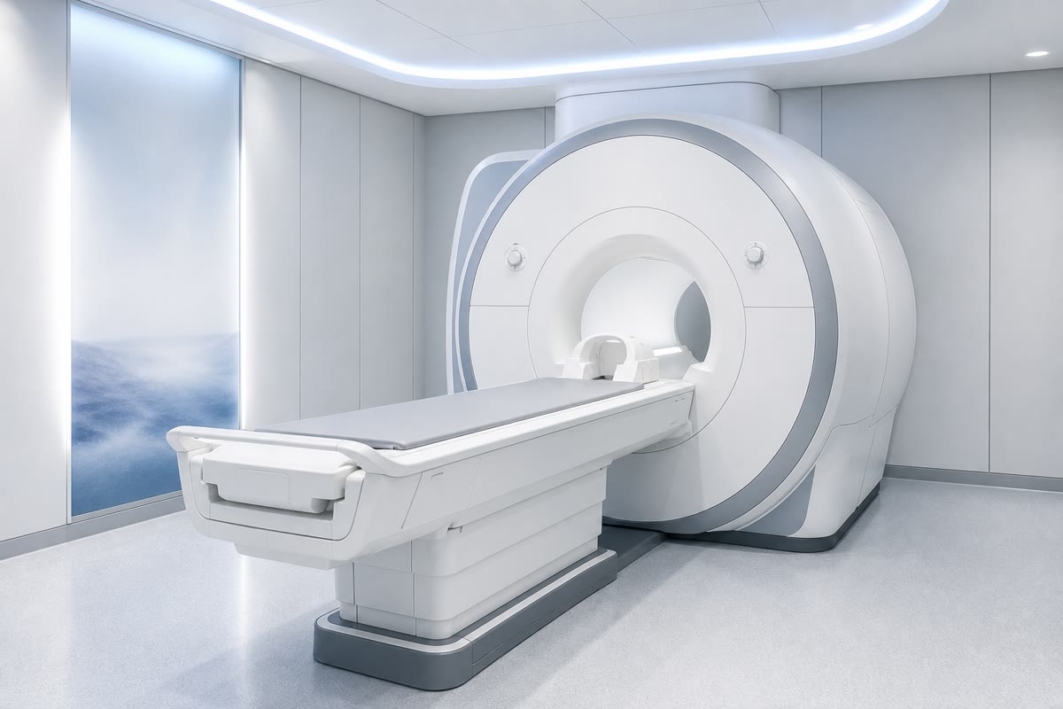
Two-thirds of a human is water; every water molecule carries two protons, each a spin- $\tfrac12$ magnet. Put a person in a strong field, tickle the protons at their Larmor frequency, and listen: that is magnetic resonance imaging, spin physics as medicine. Data: $\gamma_{\text{p}}/2\pi = 42.58\,\mathrm{MHz}/\mathrm{T}$ ; $B_0 = 3.0\,\mathrm{T}$ ; proton density of tissue $n \approx 6.6 \times 10^{28}\,\mathrm{m}^{-3}$ ; $k_{\text{B}}T$ at $310\,\mathrm{K}$ is $26.7\,\mathrm{meV}$ ; $h = 4.14 \times 10^{-15}\,\mathrm{eV}\,\mathrm{s}$ .

Part I — Spins in the magnet.

Compute the Larmor frequency at $3.0\,\mathrm{T}$ and the photon energy $h\nu$ in eV.
Compute the population imbalance between the two proton levels, $\Delta n/n \approx h\nu/2k_{\text{B}}T$ .
Only this excess — parts per million — contributes signal: how many “useful” protons per cubic centimetre of tissue?
Why is thermal polarisation so feeble here where the Stern–Gerlach beam was fully split? (What does each experiment measure: single-atom eigenvalues, or a thermal average?)
Doubling $B_0$ does what to the signal (two effects: polarisation and induced EMF at higher frequency)? Why do hospitals pay for bigger magnets?
The magnet is superconducting and always on: why is a loose steel oxygen bottle in the room a lethal projectile (which force of Example 12.1 acts on it)?

Part II — Pulses and echoes.

A transverse coil applies $B_1 = 10\,\text{µ}\mathrm{T}$ at resonance: compute the Rabi frequency and the durations of $\pi/2$ and $\pi$ pulses.
After the $\pi/2$ pulse, what does the magnetisation do, and what does Faraday’s law induce in the receiver coil (at which frequency)?
The transverse signal decays with time constant $T_2$ (spins dephase in each other’s fields and local inhomogeneities); the longitudinal magnetisation regrows with $T_1$ (energy flows to the tissue). Typical values: $T_1 \approx 1\,\mathrm{s}$ , $T_2 \approx 0.1\,\mathrm{s}$ . Why can the coherence time never much exceed the energy relaxation time (what does every energy-exchanging flip do to the phase)?
The spin echo: after the $\pi/2$ pulse and a delay $\tau$ , a $\pi$ pulse is applied and, at $2\tau$ , the dephased spins re-align and the signal returns. Explain the trick with runners on a track who are made to turn around.
Which decay does the echo undo — dephasing from static field inhomogeneities, or from fluctuating molecular fields — and why only that one?
Different tissues have different $T_1$ , $T_2$ (fat: short $T_1$ ; water/fluid: long; many tumours: longer $T_2$ than their host tissue). In one sentence: how does timing the pulse sequence turn relaxation times into image contrast?

Part III — From signal to image.

Superimpose a gradient $G = 40\,\mathrm{mT}/\mathrm{m}$ along $z$ : the Larmor frequency becomes position-dependent. Compute $\dd\nu/\dd z$ in kHz per millimetre.
A shaped RF pulse containing only the band $\nu_0 \pm 1\,\mathrm{kHz}$ excites which slab of the body? (Slice selection.)
During readout, a gradient along $x$ makes each column of the slice broadcast its own frequency: what mathematical operation turns the received time-signal into a spatial profile (recall the Fourier toolbox of the Year 2 volume)?
Estimate the total scan information: a $256 \times 256$ image at 12 bits, and why acquiring it line by line (one echo per line, repetition time $\sim T_1$ ) makes a scan take minutes.
The patient hears loud knocking: what is mechanically banging (think of the gradient coils switching in the $3\,\mathrm{T}$ field — which force)?
X-ray imaging contrasts electron density; MRI contrasts proton density and relaxation: why is MRI the tool of choice for soft tissue and the brain, and what ionising dose does it deliver?

Part IV — The spin’s other day jobs.

Chemists run the same experiment at $10\,\mathrm{ppm}$ resolution: electron clouds shield each nucleus slightly, shifting its resonance (the “chemical shift”). Why does this turn NMR into a molecular fingerprint?
Functional MRI maps thinking: deoxygenated haemoglobin is paramagnetic and shortens the local $T_2^*$ . Trace the chain from neural activity to image brightness.
The same Larmor physics with the electron’s moment runs at $84\,\mathrm{GHz}$ at $3\,\mathrm{T}$ : why is electron resonance useless inside a human but precious for studying radicals and defects?
Compare the photon energy of item 1 with typical chemical bond energies: justify the phrase “non-ionising” and contrast with a $60\,\mathrm{keV}$ X-ray photon.
The ten-ppm polarisation can be boosted: laser-polarised xenon gas reaches order-one polarisation and is inhaled to image lung airspaces. By roughly what factor does the signal per nucleus rise, and why does the gas’s low density still make the trick necessary?
A single electron spin in a silicon transistor-like trap is now read out and driven as a qubit with exactly this chapter’s pulses: name the two properties of spin (size of its Hilbert space; weakness of its coupling to noise) that recommend it.
Summarise the named result: a $128\,\mathrm{MHz}$ spin precession, a ten-parts-per-million thermal polarisation, two relaxation clocks and three field gradients suffice to photograph a living brain in slices — Stern and Gerlach’s two spots, grown into a hospital.

Solution

Solution of Problem 12.1.

1. $\nu = 42.58 \times 3.0 = 127.7\,\mathrm{MHz}$ ; $h\nu = 5.3 \times 10^{-7}\,\mathrm{eV}$ . 2. $\Delta n/n = h\nu/2k_{\text{B}}T = 5.3 \times 10^{-7}/(2 \times 0.0267) \approx 10^{-5}$ : ten parts per million. 3. $6.6 \times 10^{22}\,\mathrm{cm}^{-3} \times 10^{-5} \approx 7 \times 10^{17}$ signal-bearing protons per cubic centimetre — feeble per spin, mighty in numbers. 4. Stern–Gerlach measured each atom and split it by eigenvalue; MRI listens to a thermal average of $10^{23}$ spins, and Boltzmann keeps that average within microvolts of zero. 5. Polarisation $\propto B_0$ and the induced EMF $\propto \omega \propto B_0$ : signal roughly $\propto B_0^2$ — the case for $3\,\mathrm{T}$ over $1.5\,\mathrm{T}$ , and for the $7\,\mathrm{T}$ research machines. 6. A ferromagnet in the stray gradient feels $F = \mu\,\partial B/\partial z$ scaled to kilograms of iron: hundreds of newtons appearing in a doorway — the reason for the screening and the checklists. 7. $\nu_1 = \gamma B_1/2\pi = 426\,\mathrm{Hz}$ : $\pi/2$ pulse $0.59\,\mathrm{ms}$ , $\pi$ pulse $1.2\,\mathrm{ms}$ . 8. It precesses in the transverse plane at $127.7\,\mathrm{MHz}$ ; the rotating magnetisation’s flux through the coil induces (Faraday) a radio EMF at exactly that frequency — the raw MR signal. 9. Every energy-exchanging flip also randomises the flipped spin’s phase: whatever causes $T_1$ contributes to $T_2$ , and dephasing has extra channels of its own — coherence dies first. 10. At $\tau$ every runner turns around: the fast ones, farthest ahead, now have farthest to run back; at $2\tau$ all cross the start line abreast — the dephasing rewinds and the echo rings. 11. Only the static part: a spin that kept a constant (if wrong) frequency retraces its phase exactly; fluctuating molecular fields change between the two halves and do not rewind — their decay is the true, tissue-specific $T_2$ . 12. Sample early and often (short TR, short TE) and fat’s short $T_1$ shines; wait long and echo late and long- $T_2$ fluids glow: the sequence’s clock settings choose which relaxation constant paints the picture. 13. $\dd\nu/\dd z = 42.58\,\mathrm{MHz}/\mathrm{T} \times 0.04\,\mathrm{T}/\mathrm{m} = 1.7\,\mathrm{kHz}/\mathrm{mm}$ . 14. The slab where the local Larmor frequency falls in the band: thickness $2\,\mathrm{kHz}/1.7\,\mathrm{kHz}/\mathrm{mm} \approx 1.2\,\mathrm{mm}$ — a selected slice. 15. A Fourier transform: frequency labels position, so the spectrum of the echo is the projection of the slice. 16. $256^2 \times 12 \approx 100\,\mathrm{kB}$ ; at one encoded line per repetition time of order $T_1$ , $256$ lines cost minutes — why patients are asked to hold still. 17. The gradient coils carry kiloampere-scale switched currents inside $3\,\mathrm{T}$ : the Laplace force hammers them against their mounts at every switch — the machine-gun soundtrack of every scan. 18. X-rays shadow electron density — bone versus air — and deposit ionising dose; MRI reads proton density and two relaxation clocks, which differ richly among soft tissues: brain, cartilage and tumours, all alike to X-rays, are distinct to spins, at zero ionising dose. 19. Each chemical environment shields its proton by a few parts per million: a molecule’s protons report as a resolved comb of shifted lines — structure determination in a tube. 20. Activity raises local blood flow and oxygenation; paramagnetic deoxyhaemoglobin is diluted; local $T_2^*$ lengthens; the voxel brightens seconds after the thought. 21. At $84\,\mathrm{GHz}$ tissue is opaque (millimetre microwaves barely penetrate skin) and electron relaxation is microseconds — hopeless in vivo, but perfect for counting radicals and defects in materials and dosimetry. 22. $5 \times 10^{-7}\,\mathrm{eV}$ against eV bonds: ten million times too weak to break anything — non-ionising; one $60\,\mathrm{keV}$ X-ray photon carries $10^{11}$ times more. 23. From $10^{-5}$ to order one: a $\sim10^5$ gain per nucleus — necessary because the inhaled gas is thousands of times more dilute than water’s protons. 24. A spin- $\tfrac12$ is a perfect two-level system (no leakage levels), and it couples to charge noise only weakly through magnetic moments: long coherence in an industrial material. 25. A $128\,\mathrm{MHz}$ precession, a $10^{-5}$ polarisation, two relaxation clocks and three gradients: spin physics photographing a living brain, slice by slice, with zero ionising dose — the two silver spots of 1922 grown into a hospital department.

Terms defined in this chapter

Spin one-half

See all 431 terms in the glossary