University Physics — Year 3 · Bachelor Year 3

1Lagrangian Mechanics

Try to write Newton’s law for a double pendulum: two tension forces, neither known in advance, both changing direction at every instant, and four scalar equations to untangle just to find how two angles evolve. Now do the same for a bead on a rotating hoop, a chain of coupled springs, a robot arm. The forces that hold a system together — rods, rails, hinges — do no work, yet Newton’s method forces us to carry them through every calculation. This chapter presents the reformulation that Lagrange published in 1788: describe the system by the few coordinates that can actually change, write a single function $L = E_k - E_p$ , and one recipe produces the equations of motion in any coordinates, with every rod and rail already eliminated. Better, the new formulation makes visible what Newton’s hides: each symmetry of $L$ yields a conserved quantity — momentum from uniformity of space, energy from uniformity of time — a result of Emmy Noether that has become the organising principle of physics far beyond mechanics.

1.1 From forces to coordinates

Definition 1.1 (Constraints, degrees of freedom, generalized coordinates)

A constraint is a geometric condition imposed on the positions of a system — a bead stays on its wire, a pendulum’s rod keeps a fixed length, two wheels of an axle turn together. A constraint expressible as an equation $f(\vect r_1, \dots, \vect r_N, t) = 0$ among the coordinates (and possibly the time) is called holonomic. The number of independent ways the configuration can still vary is the number of degrees of freedom $n$ ; any set of $n$ independent quantities $q_1, \dots, q_n$ that fixes the configuration completely is a set of generalized coordinates — angles, lengths, or any convenient mixture. Their time derivatives $\dot q_1, \dots, \dot q_n$ are the generalized velocities.

Example 1.2 (Counting degrees of freedom)

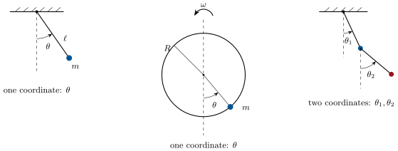
A point on a table: $n = 2$ . A plane pendulum of fixed length: one angle, $n = 1$ . A double pendulum: two angles, $n = 1 + 1 = 2$ . A bead on a rigid hoop: one angle, $n = 1$ — even if the hoop itself is forced to rotate, since the imposed rotation adds no freedom. A rigid body free in space: three coordinates of its centre plus three angles, $n = 6$ . A gas of $N$ free molecules (points): $n = 3N$ . Each holonomic constraint removes one degree of freedom: two points joined by a rod have $3 + 3 - 1 = 5$ .

Generalized coordinates: each system is described by the angles that can actually change, not by the Cartesian coordinates of its masses. The rod tensions and the hoop’s normal force never appear.

1.2 The principle of least action

Definition 1.3 (Lagrangian and action)

The Lagrangian of a mechanical system whose forces derive from a potential energy $E_p$ is the function of the coordinates, the velocities, and possibly the time

L(q, \dot q, t) = E_k - E_p ,

kinetic minus potential energy, both expressed in the generalized coordinates. The action of a conceivable motion $q(t)$ between fixed endpoints $q(t_1)$ and $q(t_2)$ is the number

S[q] = \int_{t_1}^{t_2} L\big(q(t), \dot q(t), t\big)\,\dd t .

$S$ is a functional: it eats a whole path and returns one number, in joule-seconds — the units of Planck’s constant.

Theorem 1.4 (Hamilton’s principle and the Euler–Lagrange equations)

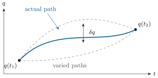
Among all conceivable motions joining the same two endpoints in the same time, the actual motion is the one that makes the action stationary (Hamilton’s principle, or the principle of least action). Equivalently, the motion obeys the Euler–Lagrange equations

\frac{\dd}{\dd t}\frac{\partial L}{\partial\dot q_i} - \frac{\partial L}{\partial q_i} = 0 , \qquad i = 1, \dots, n :

one second-order equation per degree of freedom, in whatever coordinates were chosen.

Proof. Deform the path: $q_i(t) \to q_i(t) + \delta q_i(t)$ with $\delta q_i(t_1) = \delta q_i(t_2) = 0$ . To first order,

\delta S = \int_{t_1}^{t_2}\sum_i\Big( \frac{\partial L}{\partial q_i}\,\delta q_i + \frac{\partial L}{\partial\dot q_i}\,\delta\dot q_i\Big)\dd t = \int_{t_1}^{t_2}\sum_i\Big( \frac{\partial L}{\partial q_i} - \frac{\dd}{\dd t}\frac{\partial L}{\partial\dot q_i}\Big)\delta q_i\,\dd t ,

after integrating the second term by parts ( $\delta\dot q_i = \dd(\delta q_i)/\dd t$ ) and dropping the boundary term, which vanishes at the fixed endpoints. If $\delta S = 0$ for every deformation, the bracket must vanish at every instant and for each $i$ — were it positive somewhere, a bump $\delta q_i$ concentrated there would give $\delta S \neq 0$ . The converse is read off the same line. ∎

Hamilton’s principle: among all paths with the same endpoints and duration, the actual one makes S = ∈t L\, t stationary — first-order deformations q change S only at second order. — Hamilton’s principle: among all paths with the same endpoints and duration, the actual one makes $S = \int L\,\dd t$ stationary — first-order deformations $\delta q$ change $S$ only at second order.

Proposition 1.5 (Newton recovered)

For a particle in Cartesian coordinates, $L = \tfrac12 m(\dot x^2 + \dot y^2 + \dot z^2) - E_p(x,y,z)$ , and the Euler–Lagrange equations read $m\ddot x = -\partial E_p/\partial x$ and likewise for $y$ , $z$ : exactly $m\vect a = \vect F$ . Lagrangian and Newtonian mechanics agree wherever both apply; the new form simply survives a change of coordinates, which Newton’s component equations do not.

Proof. $\partial L/\partial\dot x = m\dot x$ , $\partial L/\partial x = -\partial E_p/\partial x$ ; the Euler–Lagrange equation is $\dd(m\dot x)/\dd t + \partial E_p/\partial x = 0$ . ∎

Remark 1.6 (Why the constraint forces disappear)

The tension of a rod, the normal force of a rail, act perpendicularly to every displacement the constraint allows: they do no work in any motion compatible with the constraint. Since the action is built from energies evaluated only on such motions, these forces never enter $L$ — that is the practical miracle of the method. The general justification (d’Alembert’s principle of virtual work) is admitted here; for every system of this book the recipe below can be checked directly against Newton, as Proposition 1.5 began to do. If a constraint force is itself wanted — will the rod snap? — one returns to Newton for that force alone, with the motion already known.

Method 1.7 (The Lagrangian recipe)

(1) Count the degrees of freedom and choose coordinates $q_i$ — angles for rotations, abscissas along rails. (2) Express the positions $\vect r(q_i, t)$ , differentiate to get the velocities, and write $E_k$ ; write $E_p$ . (3) $L = E_k - E_p$ , dropping any additive constant. (4) One Euler–Lagrange equation per coordinate. (5) Before solving, harvest the conserved quantities: cyclic coordinates (Definition 1.10) and the energy function (Proposition 1.14). (6) Check limits: small angles, switched-off rotation, known special cases.

Example 1.8 (The pendulum, in three lines)

One coordinate $\theta$ ; $\vect v = \ell\dot\theta\,\vect e_\theta$ , so $E_k = \tfrac12 m\ell^2\dot\theta^2$ and $E_p = -mg\ell\cos\theta$ . Then $L = \tfrac12 m\ell^2\dot\theta^2 + mg\ell\cos\theta$ , and $\dd(m\ell^2\dot\theta)/\dd t = -mg\ell\sin\theta$ :

\ddot\theta = -\frac{g}{\ell}\sin\theta ,

the equation the Year 1 volume obtained from the torque of the weight — with the tension never mentioned.

Example 1.9 (Bead on a rotating hoop)

A bead of mass $m$ slides on a vertical circular hoop of radius $R$ forced to spin about its vertical diameter at constant $\omega$ (Example 1.2). One coordinate, the polar angle $\theta$ from the bottom. The bead’s velocity has a component $R\dot\theta$ along the hoop and $\omega R\sin\theta$ due to the imposed rotation, perpendicular to it:

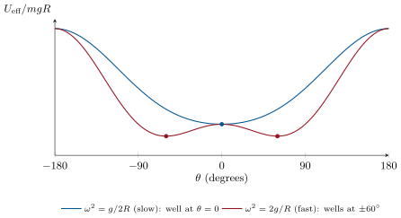
L = \tfrac12 mR^2\dot\theta^2 + \tfrac12 m\omega^2R^2\sin^2\theta + mgR\cos\theta , \qquad mR^2\ddot\theta = m\omega^2R^2\sin\theta\cos\theta - mgR\sin\theta .

Equilibria where $\ddot\theta = 0$ : the bottom $\theta = 0$ (and the top, always unstable), and, when $\omega^2 > g/R$ , a new pair $\cos\theta_{\text{eq}} = g/\omega^2R$ . Writing the equation as $mR^2\ddot\theta = -\dd U_{\text{eff}}/\dd\theta$ with the effective potential energy

U_{\text{eff}}(\theta) = -mgR\cos\theta - \tfrac12 m\omega^2R^2\sin^2\theta

makes the geometry visible: below the critical rate $\omega_{\text{c}} = \sqrt{g/R}$ the bottom is a well; above it, the bottom becomes a summit and the bead settles on the slope, climbing higher as the hoop spins faster — the principle of the centrifugal governor that regulated steam engines.

The effective potential of the bead on the rotating hoop. As crosses √g/R the single well at the bottom splits into two symmetric wells: the equilibrium angle rises with the spin rate. — The effective potential of the bead on the rotating hoop. As $\omega$ crosses $\sqrt{g/R}$ the single well at the bottom splits into two symmetric wells: the equilibrium angle rises with the spin rate.

1.3 Symmetries and conservation laws

Definition 1.10 (Generalized momentum, cyclic coordinate)

The generalized momentum conjugate to the coordinate $q_i$ is

p_i = \frac{\partial L}{\partial\dot q_i} .

For a Cartesian coordinate it is the ordinary momentum $m\dot x$ ; for an angle it is an angular momentum. A coordinate that does not appear in $L$ (though its velocity does) is called cyclic.

Proposition 1.11 (Cyclic coordinates give conservation laws)

If $q_i$ is cyclic, its conjugate momentum is conserved: $\partial L/\partial q_i = 0$ implies $\dd p_i/\dd t = 0$ . Choosing coordinates so that as many as possible are cyclic is the single most effective step in solving a mechanics problem.

Proof. Immediate from the Euler–Lagrange equation for $q_i$ . ∎

Example 1.12 (Central force, solved by inspection)

A particle in a central potential $E_p(r)$ , in polar coordinates in its plane of motion:

L = \tfrac12 m(\dot r^2 + r^2\dot\varphi^2) - E_p(r) .

$\varphi$ is cyclic, so $p_\varphi = mr^2\dot\varphi$ — the angular momentum — is conserved: Kepler’s law of areas, which the Year 1 volume derived from the torque equation, here falls out before any equation is solved. The remaining radial equation is $m\ddot r = mr\dot\varphi^2 - E_p'(r)$ , i.e. the one-dimensional motion in the effective potential $E_p(r) + p_\varphi^2/2mr^2$ of that volume.

Theorem 1.13 (Noether’s theorem)

To every continuous symmetry of the Lagrangian corresponds a conserved quantity. Precisely: if the shift $q_i \to q_i + \varepsilon\,K_i(q)$ leaves $L$ unchanged to first order in $\varepsilon$ for all motions, then

Q = \sum_i p_i\,K_i(q)

is constant along every actual motion. Uniformity of space (invariance under translation) yields momentum; isotropy of space (invariance under rotation) yields angular momentum; uniformity of time yields the energy (Proposition 1.14).

Proof. Invariance to first order means $0 = \delta L = \sum_i\big(\partial_{q_i}L\,K_i + \partial_{\dot q_i}L\,\dot K_i\big)\varepsilon$ . On an actual motion, $\partial_{q_i}L = \dot p_i$ by Euler–Lagrange, so the bracket is $\sum_i(\dot p_iK_i + p_i\dot K_i) = \dd Q/\dd t$ . A cyclic coordinate is the special case $K_i = \delta_{ij}$ . The time-shift case needs the separate computation of Proposition 1.14; the full theorem, for transformations that also change $t$ or alter $L$ by a total derivative, is proved in courses on analytical mechanics and admitted here in that generality. ∎

Proposition 1.14 (The energy function)

Along any motion, the energy function

h = \sum_i \dot q_i\,\frac{\partial L}{\partial\dot q_i} - L \qquad\text{obeys}\qquad \frac{\dd h}{\dd t} = -\frac{\partial L}{\partial t} .

If $L$ does not depend explicitly on time, $h$ is conserved. If moreover the relations $\vect r(q)$ between positions and coordinates do not involve time — no imposed rotation, no moving support — then $E_k$ is a quadratic form in the $\dot q_i$ and $h = E_k + E_p$ : the mechanical energy. With a time-dependent constraint, $h$ is still conserved when $\partial L/\partial t = 0$ , but it is not the energy: the motor enforcing the constraint exchanges work with the system.

Proof. $\dd h/\dd t = \sum_i(\ddot q_ip_i + \dot q_i\dot p_i) - \sum_i(\partial_{q_i}L\,\dot q_i + \partial_{\dot q_i}L\,\ddot q_i) - \partial_tL$ . The $\ddot q_i$ terms cancel; the Euler–Lagrange equations turn $\dot p_i$ into $\partial_{q_i}L$ , cancelling the next pair; $-\partial_tL$ remains. If $E_k = \tfrac12\sum a_{jk}(q)\dot q_j\dot q_k$ , Euler’s identity for quadratic forms gives $\sum\dot q_i\,\partial E_k/\partial\dot q_i = 2E_k$ , so $h = 2E_k - (E_k - E_p) = E_k + E_p$ . ∎

Example 1.15 (The spinning hoop keeps $h$ , not $E$ )

For the bead of Example 1.9, $L$ has no explicit $t$ , so $h = \tfrac12 mR^2\dot\theta^2 + U_{\text{eff}} (\theta)$ is conserved — but the mechanical energy $E = \tfrac12 mR^2\dot\theta^2 + \tfrac12 m\omega^2R^2\sin^2\theta - mgR\cos\theta$ is not: $E = h + m\omega^2R^2\sin^2\theta$ varies as the bead slides. The difference is the work of the motor that keeps $\omega$ constant while the bead’s distance from the axis changes.

1.4 Charged particles and small oscillations

Proposition 1.16 (Lagrangian of a charged particle)

In an electromagnetic field described by the potentials $V$ and $\vect A$ (with $\vect E = -\vect\nabla V - \partial_t\vect A$ and $\vect B = \operatorname{\vect{curl}}\vect A$ , as in the Year 2 volume), the Lagrangian

L = \tfrac12 m\vect v^{\,2} - qV + q\,\vect v\cdot\vect A

yields, through the Euler–Lagrange equations, exactly the Lorentz force $m\dot{\vect v} = q(\vect E + \vect v\wedge\vect B)$ . The magnetic force, which does no work and derives from no ordinary potential energy, enters through a term linear in the velocity; the conjugate momentum becomes $\vect p = m\vect v + q\vect A$ , no longer $m\vect v$ alone.

Proof. For the $x$ component: $p_x = m\dot x + qA_x$ , and $\partial_xL = -q\,\partial_xV + q\,\vect v\cdot\partial_x\vect A$ . The Euler–Lagrange equation gives $m\ddot x = -q\,\partial_xV - q\,\dd A_x/\dd t + q\,\vect v\cdot\partial_x\vect A$ . Along the motion $\dd A_x/\dd t = \partial_tA_x + (\vect v\cdot\vect\nabla)A_x$ , so $m\ddot x = qE_x + q\big[\vect v\cdot\partial_x\vect A - (\vect v\cdot \vect\nabla)A_x\big]$ , and the bracket is the $x$ component of $\vect v\wedge(\vect\nabla\wedge\vect A) = \vect v\wedge\vect B$ — expand both to check. ∎

Proposition 1.17 (Small oscillations and normal modes)

Near a stable equilibrium $q^{\text{eq}}$ , expand $L$ to second order in the displacements $u_i = q_i - q_i^{\text{eq}}$ : $L \approx \tfrac12\sum m_{ij}\dot u_i\dot u_j - \tfrac12\sum k_{ij}u_iu_j$ with constant symmetric matrices. The equations of motion are linear, and every motion is a superposition of normal modes: collective oscillations $u_i(t) = a_i\cos(\Omega t + \phi)$ in which all coordinates vibrate at one common frequency, the amplitudes and frequencies solving $\sum_j(k_{ij} - \Omega^2m_{ij})\,a_j = 0$ — a matrix eigenvalue problem, with $n$ modes for $n$ degrees of freedom.

Proof. Linear terms vanish at an equilibrium; the Euler–Lagrange equations of the quadratic $L$ read $\sum_jm_{ij}\ddot u_j = -\sum_jk_{ij}u_j$ . Inserting the trial oscillation gives the stated linear system, which has a nonzero amplitude vector only when $\det(k_{ij} - \Omega^2m_{ij}) = 0$ : $n$ values of $\Omega^2$ , all positive at a stable equilibrium. That the general motion is a superposition of the modes is the diagonalisation of a pair of quadratic forms, a result of the linear algebra of the Year 2 mathematics volume; completeness is admitted. ∎

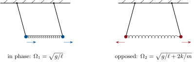
Example 1.18 (Two pendulums coupled by a spring)

Two equal pendulums (mass $m$ , length $\ell$ ), their bobs joined by a spring of stiffness $k$ relaxed when both hang straight. For small angles,

L = \tfrac12 m\ell^2(\dot\theta_1^2 + \dot\theta_2^2) - \tfrac12 mg\ell(\theta_1^2 + \theta_2^2) - \tfrac12 k\ell^2(\theta_2 - \theta_1)^2 .

Symmetry suggests the combinations $s = \theta_1 + \theta_2$ and $d = \theta_1 - \theta_2$ , which decouple the equations: the in-phase mode ( $\theta_1 = \theta_2$ , spring inert) at $\Omega_1 = \sqrt{g/\ell}$ , and the opposed mode ( $\theta_1 = -\theta_2$ , spring stretched twice) at $\Omega_2 = \sqrt{g/\ell + 2k/m}$ . Start one pendulum alone — an equal mixture of the two modes — and the energy migrates entirely from one pendulum to the other and back at the beat frequency $(\Omega_2 - \Omega_1)/2\pi$ : the coupled-pendulum demonstration, and the mechanism behind every resonant energy transfer from tuned circuits to molecular vibrations.

The two normal modes of the coupled pendulums. In phase, the spring never stretches and the frequency is the free pendulum’s; opposed, each bob feels the spring doubled.

A double pendulum traced by a long exposure: two coordinates, one Lagrangian, and a motion no formula predicts for long — the least-action machinery of this chapter writes the equations; chaos keeps their solutions humble.

1.5 Exercises

Exercise 1.1 ★

Count the degrees of freedom and propose generalized coordinates: (a) a particle on the inside of a fixed bowl; (b) a cylinder rolling without slipping down a fixed incline; (c) a double pendulum whose upper pivot slides on a horizontal rail; (d) a dumbbell (two masses, rigid rod) in space; (e) two beads on the same fixed circular wire. Which constraint in this list relates velocities rather than positions, and why is it nevertheless integrable to a holonomic one?

Solution

Solution of Exercise 1.1.

(a) 2 (two angles on the bowl’s surface). (b) 1: the abscissa $x$ along the slope, the rotation angle being tied to it by rolling, $x = R\phi$ . (c) 3: $X$ , $\theta_1$ , $\theta_2$ . (d) 5: three for the centre, two for the rod’s direction. (e) 2: one angle each. The rolling condition is a relation between velocities, $\dot x = R\dot\phi$ ; in this plane problem it integrates at once to $x = R\phi + \text{const}$ , hence holonomic. (For a ball rolling on a plane it does not integrate, and Lagrangian mechanics needs an extension.)

Exercise 1.2 ★

For the plane pendulum (Example 1.8): (a) verify the dimensions of $L$ and of $p_\theta = \partial L/\partial\dot\theta$ ; (b) identify $p_\theta$ physically; (c) derive the small-angle period; (d) compute the action $S$ of one full small oscillation of amplitude $\theta_0$ — and explain the answer before computing (what is the time average of $E_k - E_p$ for a harmonic oscillation?).

Solution

Solution of Exercise 1.2.

(a) $[L] = \mathrm{J}$ ; $[p_\theta] = \mathrm{kg}\,\mathrm{m}^{2}/\mathrm{s}$ — an angular momentum, since $\theta$ is dimensionless. (b) $p_\theta = m\ell^2\dot\theta$ is the angular momentum of the bob about the pivot. (c) $\ddot\theta = -(g/\ell)\theta$ gives $T = 2\pi\sqrt{\ell/g}$ . (d) With $E_p$ measured from the equilibrium, a harmonic oscillation has equal time-averaged kinetic and potential energies, so $\langle L\rangle = 0$ and $S = 0$ over a whole period — the computation confirms it: $S = \int_0^T\tfrac12 m\ell^2\theta_0^2[\omega^2\sin^2 \omega t - (g/\ell)\cos^2\omega t]\,\dd t = 0$ since $\omega^2 = g/\ell$ .

Exercise 1.3 ★

An Atwood machine: masses $m_1$ and $m_2$ hang from an ideal string over a massless pulley. (a) Choose one coordinate and write $L$ . (b) Find the acceleration. (c) Newton’s treatment needed the tension — where did it go? (d) How would you recover the tension once the motion is known?

Solution

Solution of Exercise 1.3.

(a) Let $x$ be the descent of $m_1$ (so $m_2$ rises by $x$ ): $L = \tfrac12(m_1 + m_2)\dot x^2 + (m_1 - m_2)gx$ . (b) $(m_1 + m_2)\ddot x = (m_1 - m_2)g$ : $a = (m_1 - m_2)g/(m_1 + m_2)$ . (c) The tension acts at both ends of an inextensible string: in any allowed displacement its works cancel, so it never enters $L$ . (d) Newton on $m_1$ alone: $T = m_1(g - a) = 2m_1m_2g/(m_1 + m_2)$ .

Exercise 1.4 ★

A free particle in cylindrical coordinates: $L = \tfrac12 m(\dot r^2 + r^2\dot\varphi^2 + \dot z^2)$ . (a) Which coordinates are cyclic, and what are the conserved momenta? (b) Why is $p_r$ not conserved even though no force acts? (c) Write the Euler–Lagrange equation for $r$ and interpret the term $mr\dot\varphi^2$ . (d) Check that a straight line traversed at constant speed solves it.

Solution

Solution of Exercise 1.4.

(a) $\varphi$ and $z$ : $p_\varphi = mr^2\dot\varphi$ (angular momentum about the axis) and $p_z = m\dot z$ are conserved. (b) $r$ appears in $L$ through $r^2\dot\varphi^2$ , so it is not cyclic: $\dot p_r = mr\dot\varphi^2 \neq 0$ . Nothing is wrong — $p_r = m\dot r$ is the radial component of a constant vector $\vect p$ , and a component along a turning direction need not be constant. (c) $m\ddot r = mr\dot\varphi^2$ : the centrifugal term, the price of using coordinates attached to directions that rotate. (d) For a line at distance $b$ passed at speed $v$ : $r = \sqrt{b^2 + v^2t^2}$ , $r^2\dot\varphi = bv$ ; then $\ddot r = b^2v^2/r^3 = r(bv/r^2)^2 = r\dot\varphi^2$ .

Exercise 1.5 ★★

A block of mass $m$ slides on the frictionless face (angle $\alpha$ ) of a wedge of mass $M$ , itself free to slide on a frictionless floor. (a) Choose two coordinates: the wedge’s abscissa $X$ and the block’s distance $s$ down the face; write $L$ . (b) Which coordinate is cyclic, and what conservation law does it express? (c) Find the two accelerations. (d) Check the limits $M \to \infty$ and $\alpha \to 90^\circ$ .

Solution

Solution of Exercise 1.5.

(a) Block position $(X + s\cos\alpha,\ -s\sin\alpha)$ , so

L = \tfrac12 M\dot X^2 + \tfrac12 m\big(\dot X^2 + 2\dot X\dot s\cos\alpha + \dot s^2\big) + mgs\sin\alpha .

(b) $X$ is cyclic: $P = (M + m)\dot X + m\dot s\cos\alpha$ is conserved — the total horizontal momentum, since no external horizontal force acts. (c) The $s$ equation is $\ddot s + \ddot X\cos\alpha = g\sin\alpha$ ; with $\ddot X = -m\ddot s\cos\alpha/(M + m)$ from (b),

\ddot s = \frac{(M + m)g\sin\alpha}{M + m\sin^2\alpha} , \qquad \ddot X = -\frac{mg\sin\alpha\cos\alpha}{M + m\sin^2\alpha} .

(d) $M \to \infty$ : $\ddot s \to g\sin\alpha$ , the fixed incline; $\alpha \to 90^\circ$ : $\ddot s \to g$ , $\ddot X \to 0$ — free fall along a vertical face, the wedge unpushed.

Exercise 1.6 ★★

The spherical pendulum: a bob on a rod of length $\ell$ , free in both angles ( $\theta$ from the downward vertical, $\varphi$ around it). (a) Write $L$ . (b) Identify the cyclic coordinate and the conserved $p_\varphi$ . (c) Reduce the motion of $\theta$ to an effective potential and sketch it. (d) For the conical motion $\theta = \theta_0$ , recover the conical-pendulum relation $\cos\theta_0 = g/\ell\omega^2$ of the Year 1 volume.

Solution

Solution of Exercise 1.6.

(a) $L = \tfrac12 m\ell^2(\dot\theta^2 + \sin^2\theta\,\dot\varphi^2) + mg\ell\cos\theta$ . (b) $\varphi$ cyclic: $p_\varphi = m\ell^2\sin^2\theta\,\dot\varphi$ , the vertical angular momentum. (c) Eliminating $\dot\varphi$ , $\tfrac12 m\ell^2\dot\theta^2 + U_{\text{eff}}(\theta)$ is conserved with

U_{\text{eff}}(\theta) = \frac{p_\varphi^2}{2m\ell^2\sin^2\theta} - mg\ell\cos\theta :

a wall at $\theta = 0$ and $\theta = \pi$ (for $p_\varphi \neq 0$ ) with one minimum between — the bob nutates between two circles. (d) At the minimum, $\dot\theta = 0$ with $\theta = \theta_0$ constant: $p_\varphi^2\cos\theta_0/m\ell^2\sin^3\theta_0 = mg\ell\sin\theta_0$ ; inserting $p_\varphi = m\ell^2\sin^2\theta_0\,\omega$ gives $\ell\omega^2\cos\theta_0 = g$ .

Exercise 1.7 ★★

A pendulum (mass $m$ , length $\ell$ ) hangs from a cart of mass $M$ free to roll on a horizontal rail. (a) With coordinates $X$ (cart) and $\theta$ , write $L$ . (b) What is conserved, and why physically? (c) Linearise for small $\theta$ and show that the oscillation frequency is $\Omega = \sqrt{(1 + m/M)\,g/\ell}$ . (d) Explain the limits $M \to \infty$ and $M \to 0$ — why does a light cart raise the frequency?

Solution

Solution of Exercise 1.7.

(a) Bob at $(X + \ell\sin\theta,\ -\ell\cos\theta)$ :

L = \tfrac12(M + m)\dot X^2 + m\ell\cos\theta\,\dot X\dot\theta + \tfrac12 m\ell^2\dot\theta^2 + mg\ell\cos\theta .

(b) $X$ cyclic: $(M + m)\dot X + m\ell\cos\theta\,\dot\theta$ is conserved — the horizontal momentum of the whole system (the rail pushes only vertically). (c) Small angles: $(M + m)\ddot X + m\ell\ddot\theta = 0$ and $\ell\ddot\theta + \ddot X + g\theta = 0$ ; eliminating $\ddot X$ , $\ell\ddot\theta\,[1 - m/(M + m)] = -g\theta$ , so $\Omega^2 = (M + m)g/M\ell = (1 + m/M)\,g/\ell$ . (d) $M \to \infty$ : the fixed pivot, $\Omega^2 = g/\ell$ . Small $M$ : the cart recoils opposite to the bob, the pivot-to-bob swing happens about a point between them (the fixed centre of mass), shortening the effective pendulum — hence the higher frequency, diverging as $M \to 0$ .

Exercise 1.8 ★★

A particle of charge $q$ in a uniform field $\vect B = B\vect e_z$ , described by $\vect A = \tfrac12\vect B\wedge\vect r$ . (a) Write $L$ in Cartesian coordinates. (b) Derive the equations of motion and check they describe the cyclotron circle at $\omega_{\text{c}} = qB/m$ . (c) Compute the conjugate momenta $p_x$ , $p_y$ : are they $m\dot x$ , $m\dot y$ ? Are they conserved? (d) Show that $L$ written in cylindrical coordinates has $\varphi$ cyclic, and identify the conserved $p_\varphi$ for a circle centred on the axis.

Solution

Solution of Exercise 1.8.

(a) $\vect A = \tfrac12 B(-y, x, 0)$ : $L = \tfrac12 m(\dot x^2 + \dot y^2 + \dot z^2) + \tfrac12 qB(x\dot y - y\dot x)$ . (b) The $x$ equation: $\dd(m\dot x - \tfrac12 qBy)/\dd t = \tfrac12 qB\dot y$ , i.e. $m\ddot x = qB\dot y$ ; likewise $m\ddot y = -qB\dot x$ : circular motion at $\omega_{\text{c}} = qB/m$ , $\dot z$ constant. (c) $p_x = m\dot x - \tfrac12 qBy \neq m\dot x$ ; neither $x$ nor $y$ is cyclic ( $\partial L/\partial x = \tfrac12 qB\dot y$ ), so neither momentum is conserved — only combinations like $m\dot x - qBy$ are (check: its derivative vanishes). (d) In cylindrical coordinates $A_\varphi = \tfrac12 Br$ : $L = \tfrac12 m(\dot r^2 + r^2\dot\varphi^2 + \dot z^2) + \tfrac12 qBr^2\dot\varphi$ ; $\varphi$ is cyclic, $p_\varphi = mr^2\dot\varphi + \tfrac12 qBr^2$ . On a circle of radius $R$ centred on the axis, $\dot\varphi = -\omega_{\text{c}}$ , so $p_\varphi = -qBR^2 + \tfrac12 qBR^2 = -\tfrac12 qBR^2$ .

Exercise 1.9 ★★

For the bead on the rotating hoop (Example 1.9): (a) compute the energy function $h$ and verify it is conserved by the equation of motion; (b) compute the mechanical energy $E$ and show $E - h = m\omega^2R^2\sin^2\theta$ ; (c) find the power delivered by the motor as a function of $\theta$ and $\dot\theta$ ; (d) find the frequency of small oscillations about the tilted equilibrium when $\omega^2 > g/R$ , and show it vanishes as $\omega^2 \to g/R$ — the slowing down that announces the split of the well.

Solution

Solution of Exercise 1.9.

(a) $h = \dot\theta\,\partial L/\partial\dot\theta - L = \tfrac12 mR^2\dot\theta^2 - \tfrac12 m\omega^2R^2\sin^2\theta - mgR\cos\theta = \tfrac12 mR^2\dot\theta^2 + U_{\text{eff}}$ ; $\dd h/\dd t = \dot\theta\,[mR^2\ddot\theta + U_{\text{eff}}'(\theta)] = 0$ by the equation of motion. (b) $E = \tfrac12 mR^2\dot\theta^2 + \tfrac12 m\omega^2R^2\sin^2\theta - mgR\cos\theta = h + m\omega^2R^2\sin^2\theta$ . (c) $P = \dd E/\dd t = m\omega^2R^2\sin2\theta\,\dot\theta$ : positive while the bead climbs away from the axis (the motor works against the bead’s inertia), negative on the way back. (d) $U_{\text{eff}}'' = mgR\cos\theta - m\omega^2R^2\cos2\theta$ ; at $\cos\theta_{\text{eq}} = g/\omega^2R$ this is $m\omega^2R^2\sin^2\theta_{\text{eq}}$ , so $\omega_{\text{osc}} = \omega\sin\theta_{\text{eq}} = \omega\sqrt{1 - (g/\omega^2R)^2} \to 0$ as $\omega^2 \to g/R$ : the restoring force flattens exactly when the wells merge.

Exercise 1.10 ★★★

The equal double pendulum ( $m_1 = m_2 = m$ , $\ell_1 = \ell_2 = \ell$ ). (a) Show that for small angles $L = \tfrac12 m\ell^2(2\dot\theta_1^2 + 2\dot\theta_1\dot\theta_2 + \dot\theta_2^2) - \tfrac12 mg\ell(2 \theta_1^2 + \theta_2^2)$ . (b) Write the two equations of motion. (c) Find the normal frequencies $\Omega_\pm^2 = (2 \mp \sqrt2)\,g/\ell$ and the shape of each mode ( $\theta_2 = \pm\sqrt2\,\theta_1$ ). (d) At large amplitude this system is a standard example of chaos: explain in a few lines what breaks the small-angle analysis, and why no conservation law is lost.

Solution

Solution of Exercise 1.10.

(a) Positions $x_2 = \ell(\sin\theta_1 + \sin\theta_2)$ , etc.; keeping quadratic terms, the cross velocity term is $m\ell^2\dot\theta_1\dot\theta_2$ , giving the stated $L$ . (b) $2\ddot\theta_1 + \ddot\theta_2 = -2\omega_0^2\theta_1$ and $\ddot\theta_1 + \ddot\theta_2 = -\omega_0^2\theta_2$ , with $\omega_0^2 = g/\ell$ . (c) Inserting $\theta_i = a_i\cos\Omega t$ : $\det\begin{pmatrix} 2\omega_0^2 - 2\Omega^2 & -\Omega^2\\ -\Omega^2 & \omega_0^2 - \Omega^2\end{pmatrix} = \Omega^4 - 4\omega_0^2\Omega^2 + 2\omega_0^4 = 0$ , so $\Omega_\pm^2 = (2 \mp \sqrt2)\omega_0^2$ ; the second line gives $a_2/a_1 = \Omega^2/(\omega_0^2 - \Omega^2) = \pm\sqrt2$ : bobs together (slow mode), bobs opposed (fast mode). (d) At large amplitude the $\sin$ and $\cos$ couplings make the equations nonlinear; solutions no longer superpose, and neighbouring initial conditions separate exponentially (chaos). Energy is still exactly conserved — $L$ has no explicit time — chaos is about predictability, not conservation.

Exercise 1.11 ★★★

The brachistochrone. A bead slides without friction from rest at the origin down a curve $y(x)$ ( $y$ downward) to a point $(a, b)$ . (a) Using energy conservation, show the descent time is $T = \int_0^a\sqrt{(1 + y'^2)/2gy}\,\dd x$ — a functional, with $x$ playing the role of time. (b) The integrand $F(y, y')$ has no explicit $x$ : show that $h = y'\,\partial F/\partial y' - F$ is constant along the optimal curve (the same computation as Proposition 1.14). (c) Deduce $y(1 + y'^2) = 2r$ for a constant $r$ , and verify that the cycloid $x = r(\phi - \sin\phi)$ , $y = r(1 - \cos\phi)$ satisfies it. (d) Show the bead’s descent to the bottom of one arch takes $\pi\sqrt{r/g}$ , and compare with the straight chute to the same point.

Solution

Solution of Exercise 1.11.

(a) $v = \sqrt{2gy}$ and $\dd s = \sqrt{1 + y'^2}\,\dd x$ give the functional. (b) The computation of Proposition 1.14 with $x$ for time: $\dd h/\dd x = -\partial F/\partial x = 0$ . (c) $h = -1/\sqrt{2gy(1 + y'^2)}$ , so $y(1 + y'^2) = 2r$ . For the cycloid, $y' = \sin\phi/(1 - \cos\phi)$ and $1 + y'^2 = 2/(1 - \cos\phi)$ , hence $y(1 + y'^2) = 2r$ . (d) $\dd t = \dd s/v = \sqrt{r/g}\,\dd\phi$ (all $\phi$ -dependence cancels), so the bottom ( $\phi = \pi$ ) is reached in $\pi\sqrt{r/g}$ — whatever the starting point: the cycloid is also the tautochrone. The straight chute to $(\pi r, 2r)$ takes $\sqrt{\pi^2 + 4}\,\sqrt{r/g} \approx 3.72\sqrt{r/g}$ , about $18\%$ longer than $\pi\sqrt{r/g}$ .

Exercise 1.12 ★★★

Fermat as least action. Light in a medium of index $n(y)$ travels between two points in the least time (Year 2 volume). (a) Show the travel time along $y(x)$ is $T = \tfrac1c\int n(y)\sqrt{1 + y'^2}\,\dd x$ . (b) Since the integrand has no explicit $x$ , use the conserved $h$ of the previous exercise to show $n(y)\big/\sqrt{1 + y'^2} = \text{const}$ , and check this is Snell’s law $n\sin i = \text{const}$ for a ray measured from the vertical. (c) Over a hot road the index grows with height as $n(y) \approx n_0(1 + \beta y)$ ; show a nearly horizontal ray bends with curvature radius $R \approx 1/\beta$ . (d) With $\beta = 1.2 \times 10^{-5}\,\mathrm{m}^{-1}$ , from what distance does a driver whose eyes are $1.2\,\mathrm{m}$ above the road see the “water” mirage on it?

Solution

Solution of Exercise 1.12.

(a) $\dd t = \dd s/(c/n)$ . (b) $h = -n(y)/\sqrt{1 + y'^2}$ is conserved; $1/\sqrt{1 + y'^2} = \cos\theta$ ( $\theta$ the slope angle) $= \sin i$ for $i$ from the vertical: $n\sin i = \text{const}$ — Snell’s law, continuously applied. (c) For a nearly horizontal ray $n\cos\theta \approx \text{const}$ with $\theta$ small gives $\theta\,\dd\theta = \dd n/n \approx \beta\,\dd y$ ; since $\dd y = \theta\,\dd x$ , the curvature is $\dd\theta/\dd x = \beta$ , i.e. $R = 1/\beta \approx 83\,\mathrm{km}$ , bending upward (toward larger $n$ ). (d) A ray from the eye, tangent to the road after curving with radius $R$ , touches it at $d = \sqrt{2hR} = \sqrt{2 \times 1.2 \times 8.3e4} \approx 450\,\mathrm{m}$ : beyond that distance the road itself is not seen — one sees sky refracted upward, the shimmering “water”.

Foucault’s pendulum in the Panthéon, Paris. Generalised coordinates, a constraint, and a slowly turning frame: the room’s rotation appears in the equations of motion — and the swing plane’s drift lets a basement measure the Earth’s spin. Photograph: Olga Khomitsevich, CC BY 2.0.

1.6 Problem: The broom that stands upside down

Problem 1.1

Weekend problem — Kapitza’s inverted pendulum

A rigid pendulum can stand stably above its pivot if the pivot is shaken up and down fast enough — a discovery analysed by Kapitza in 1951, striking enough to look like a conjuring trick, and the principle by which oscillating electric fields trap single ions. We model the pendulum as a point mass $m$ at the end of a massless rigid rod of length $\ell = 40\,\mathrm{cm}$ ; $\theta$ is the angle from the downward vertical; $g = 9.81\,\mathrm{m}/\mathrm{s}^{2}$ .

Part I — The rigid pendulum. The pivot is first held fixed.

Write the Lagrangian and the equation of motion.
Give the frequency $f_0$ of small oscillations about $\theta = 0$ , and its value.
Show that $h = E$ here, and use its conservation to find the minimum launch speed of the bob, at the bottom, that carries it to the top.
Linearise the equation near $\theta = \pi$ (set $\theta = \pi + \epsilon$ ) and show $\ddot\epsilon = +(g/\ell)\epsilon$ : how fast does an initial millidegree of tilt grow? Give the time for it to grow by a factor $e$ .
A broom balanced on a fingertip falls in about a second, yet never stands alone: state in one sentence what the linearised equation says about the equilibrium $\theta = \pi$ .

Part II — Shaking the pivot. The pivot now oscillates vertically, its height $y_{\text{s}}(t) = a\cos\Omega t$ with $a = 2.0\,\mathrm{cm}$ , $\Omega$ adjustable.

Write the coordinates of the bob and show $\vect v^{\,2} = \ell^2\dot\theta^2 - 2a\Omega\ell\sin(\Omega t)\sin\theta\,\dot\theta + a^2\Omega^2\sin^2\Omega t$ .
Show that two Lagrangians differing by a total time derivative $\dd F(q,t)/\dd t$ give the same Euler–Lagrange equations.
Using this freedom, reduce the Lagrangian to $L = \tfrac12 m \ell^2\dot\theta^2 - ma\Omega^2\ell\cos(\Omega t)\cos\theta + mg\ell\cos\theta$ . (Hint: $\sin(\Omega t)\sin\theta\,\dot\theta$ combines with a $\cos(\Omega t)\cos\theta$ term into a total derivative; terms in $t$ alone may be dropped.)
Derive the equation of motion

$\ddot\theta = -\frac{g}{\ell}\sin\theta + \frac{a\Omega^2}{\ell}\cos(\Omega t)\sin\theta .$

Interpret the second term as the weight being replaced by $g + \ddot y_{\text{s}}$ : the pendulum lives in an elevator.
Is the energy function $h$ conserved now? Is the energy? What pumps energy in and out?
In Kapitza’s regime $a \ll \ell$ and $\Omega \gg \omega_0 = \sqrt{g/\ell}$ : check these for $a = 2\,\mathrm{cm}$ , $\ell = 40\,\mathrm{cm}$ , $\Omega/2\pi = 40\,\mathrm{Hz}$ , and explain physically why the bob then cannot follow the drive.

Part III — Separating fast from slow. Seek the motion as $\theta(t) = \Theta(t) + \xi(t)$ : a slow drift $\Theta$ plus a small ripple $\xi$ at the drive frequency.

Keeping only the largest term on each side, show the ripple obeys $\ddot\xi \approx +(a\Omega^2/\ell)\cos(\Omega t) \sin\Theta$ , with $\Theta$ frozen on the drive timescale.
Deduce $\xi(t) = -(a/\ell)\cos(\Omega t)\sin\Theta$ , and check that its amplitude is small, of order $a/\ell$ .
Expand $\sin\theta = \sin(\Theta + \xi)$ to first order in $\xi$ and insert it into the equation of motion.
Average over one drive period, with $\Theta$ held fixed: using $\langle\cos\Omega t\rangle = 0$ and $\langle\cos^2\Omega t\rangle = \tfrac12$ , show

$\ddot\Theta = -\frac{g}{\ell}\sin\Theta - \frac{a^2\Omega^2}{2\ell^2}\sin\Theta\cos\Theta .$
Show this is motion in the effective potential

$U_{\text{eff}}(\Theta) = mg\ell\Big({-\cos\Theta} + \frac{a^2\Omega^2}{4g\ell}\sin^2\Theta\Big) .$
Compare with the bead on the rotating hoop (Example 1.9): same mathematics, opposite sign of the new term — what does the shaking do to the bottom equilibrium that the rotation did not?
Sketch $U_{\text{eff}}$ for slow and for fast drive, and describe every equilibrium and its stability in each case.

Part IV — The broom stands up.

Expanding $U_{\text{eff}}$ near $\Theta = \pi$ , show the inverted position is stable exactly when

$a^2\Omega^2 > 2g\ell .$
Compute the critical drive frequency $f_{\text{c}} = \Omega_{\text{c}}/2\pi$ for our pendulum, and the peak pivot speed $a\Omega_{\text{c}}$ and acceleration $a\Omega_{\text{c}}^2$ (in units of $g$ ) it demands.
At $\Omega = 2\Omega_{\text{c}}$ , find the frequency of the slow swaying of the standing pendulum about $\Theta = \pi$ , and its value; check it is indeed slow compared with the drive.
Still at $\Omega = 2\Omega_{\text{c}}$ , what is the ripple amplitude $\xi$ at $\Theta$ slightly off $\pi$ , in degrees, for $a/\ell = 0.05$ ? Would a photograph betray the trick?
How far from the vertical may the broom lean and still return? Show the standing well extends over $|\Theta - \pi| < \arccos(2g\ell/a^2\Omega^2)$ , and evaluate it at $\Omega = 2\Omega_{\text{c}}$ .
A juggler balancing a broom on a still fingertip also keeps it up — by what entirely different mechanism? Name the feature of Kapitza’s pendulum that needs no feedback.
Summarise the named result: a pivot shaken with amplitude $2\,\mathrm{cm}$ at $45\,\mathrm{Hz}$ — twice the critical frequency — holds a $40\,\mathrm{cm}$ pendulum upside down, in a well reaching some $75^\circ$ from the vertical, swaying gently at about $1.4\,\mathrm{Hz}$ . Where in physics is the same averaged trapping used to hold a single charged particle?

Solution

Solution of Problem 1.1.

1. $L = \tfrac12 m\ell^2\dot\theta^2 + mg\ell\cos\theta$ ; $\ddot\theta = -(g/\ell)\sin\theta$ . 2. $f_0 = \sqrt{g/\ell}/2\pi = 0.79\,\mathrm{Hz}$ . 3. The suspension is fixed, so $h = E = \tfrac12 m\ell^2\dot\theta^2 - mg\ell\cos\theta$ ; from bottom to top $\tfrac12 mv^2 = 2mg\ell$ : $v = 2\sqrt{g\ell} = 4.0\,\mathrm{m}/\mathrm{s}$ . 4. $\ddot\epsilon = +(g/\ell)\epsilon$ : $\epsilon \propto \eu^{t/\tau}$ with $\tau = \sqrt{\ell/g} = 0.20\,\mathrm{s}$ . 5. The inverted equilibrium exists but is exponentially unstable: any tilt, however small, multiplies by $e$ every $0.2\,\mathrm{s}$ . 6. Bob at $(\ell\sin\theta,\ a\cos\Omega t - \ell\cos\theta)$ ; differentiate and square: the stated $\vect v^{\,2}$ , with the cross term $-2a\Omega\ell\sin(\Omega t)\sin\theta\,\dot\theta$ . 7. If $L' = L + \dd F(q,t)/\dd t$ , the action changes by $F(q_2, t_2) - F(q_1, t_1)$ , a constant under variations with fixed endpoints: same stationary paths, same equations. 8. The cross term is $-ma\Omega\ell\sin(\Omega t)\sin\theta\, \dot\theta = \dd[ma\Omega\ell\sin(\Omega t)\cos\theta]/\dd t - ma\Omega^2\ell\cos(\Omega t)\cos\theta$ ; dropping the total derivative and the terms in $t$ alone ( $\tfrac12 ma^2\Omega^2\sin^2\Omega t$ and $-mga\cos\Omega t$ ) leaves the stated $L$ . 9. $m\ell^2\ddot\theta = -mg\ell\sin\theta + ma\Omega^2\ell\cos(\Omega t)\sin\theta$ . Since $\ddot y_{\text{s}} = -a\Omega^2\cos\Omega t$ , this is $\ddot\theta = -[(g + \ddot y_{\text{s}})/\ell]\sin\theta$ : in the pivot’s frame the apparent gravity oscillates. 10. $L$ now depends explicitly on $t$ : $h$ is not conserved, nor is $E$ — the shaker feeds energy in and out through the pivot. 11. $a/\ell = 0.05$ ; $\Omega = 251\,\mathrm{rad}/\mathrm{s}$ against $\omega_0 = 4.9\,\mathrm{rad}/\mathrm{s}$ : ratio $51$ . In one drive period ( $25\,\mathrm{ms}$ ) gravity barely changes $\dot\theta$ : the bob is too sluggish to follow, and only quivers. 12. $\ddot\xi$ is the largest derivative ( $\propto\Omega^2$ ) and the drive the largest force term: $\ddot\xi = (a\Omega^2/\ell)\cos(\Omega t)\sin\Theta$ . 13. Integrating twice at fixed $\Theta$ : $\xi = -(a/\ell)\cos(\Omega t)\sin\Theta$ , of amplitude at most $a/\ell = 0.05$ : a two-degree quiver. 14. $\sin\theta \approx \sin\Theta + \xi\cos\Theta$ , so

\ddot\Theta + \ddot\xi = -\frac{g}{\ell}(\sin\Theta + \xi\cos\Theta) + \frac{a\Omega^2}{\ell}\cos\Omega t\,(\sin\Theta + \xi\cos\Theta) .

15. Averaging kills $\ddot\xi$ , $\langle\cos\Omega t\rangle$ and $\langle\xi\rangle$ ; the surviving cross term is $(a\Omega^2/\ell)\cos\Theta\,\langle\xi\cos\Omega t\rangle = -(a^2\Omega^2/2\ell^2)\sin\Theta\cos\Theta$ , giving the stated equation for $\Theta$ . 16. $\ddot\Theta = -(1/m\ell^2)\,U_{\text{eff}}'(\Theta)$ with $U_{\text{eff}} = mg\ell[-\cos\Theta + (a^2\Omega^2/4g\ell) \sin^2\Theta]$ — differentiate to check. 17. Same $\sin^2$ term as the hoop’s but with the opposite sign: rotation dug wells on the flanks and could only flatten the bottom; vertical shaking stiffens the bottom well and digs a new well at the top. 18. Slow drive ( $a^2\Omega^2 < 2g\ell$ ): minimum at $\Theta = 0$ , maximum at $\pi$ — nothing new. Fast drive: minima at $0$ and $\pi$ , separated by maxima at $\cos\Theta^* = -2g\ell/a^2\Omega^2$ ; both hanging and standing pendulums oscillate stably. 19. Near $\pi$ , with $\Theta = \pi + \epsilon$ : $\ddot\epsilon = [g/\ell - a^2\Omega^2/2\ell^2]\,\epsilon$ ; stability requires the bracket negative: $a^2\Omega^2 > 2g\ell$ . 20. $\Omega_{\text{c}} = \sqrt{2g\ell}/a = 140\,\mathrm{rad}/\mathrm{s}$ : $f_{\text{c}} = 22\,\mathrm{Hz}$ ; peak speed $a\Omega_{\text{c}} = 2.8\,\mathrm{m}/\mathrm{s}$ , peak acceleration $a\Omega_{\text{c}}^2 = 392\,\mathrm{m}/\mathrm{s}^{2} \approx 40g$ . 21. $\omega_{\text{slow}} = \sqrt{a^2\Omega^2/2\ell^2 - g/\ell}$ ; at $\Omega = 2\Omega_{\text{c}}$ , $a^2\Omega^2 = 8g\ell$ so $\omega_{\text{slow}} = \sqrt{3g/\ell} = 8.6\,\mathrm{rad}/\mathrm{s}$ : $1.4\,\mathrm{Hz}$ , thirty times slower than the $45\,\mathrm{Hz}$ drive. 22. $\xi_{\max} = (a/\ell)\sin\Theta$ : leaning $10^\circ$ off the vertical, $\xi_{\max} = 0.05\sin170^\circ = 8.7\,\mathrm{mrad} \approx 0.5^\circ$ — an ordinary photograph shows a broom standing still. 23. The standing well reaches the flanking maxima: $|\Theta - \pi| < \arccos(2g\ell/a^2\Omega^2)$ ; at $\Omega = 2\Omega_{\text{c}}$ , $\arccos\tfrac14 = 75^\circ$ — a remarkably forgiving well. 24. The juggler uses feedback: eyes measure the tilt, the hand accelerates sideways to cancel it. Kapitza’s stabilisation is open-loop — the drive never knows where the pendulum is. 25. Shaken at $45\,\mathrm{Hz}$ with $2\,\mathrm{cm}$ amplitude, the $40\,\mathrm{cm}$ pendulum stands inverted in a $75^\circ$ well, swaying at $1.4\,\mathrm{Hz}$ . The same time-averaged effective potential, made with an oscillating electric quadrupole field instead of a shaken pivot, confines single ions in the Paul trap — the workhorse of atomic clocks and trapped-ion quantum computing.

Terms defined in this chapter

See all 431 terms in the glossary