University Physics — Year 3 · Bachelor Year 3

17The Canonical Ensemble

Isolated systems are a theorist’s fiction: real samples sit in thermostats, rooms, oceans of air — in contact with a reservoir that fixes not their energy but their temperature. The Year 2 volume met the resulting law empirically: the probability of a state of energy $E$ carries the factor $\eu^{-E/k_{\text{B}}T}$ . This chapter derives that Boltzmann factor in four lines from the counting of Chapter 16, then builds the machine that makes statistical physics an industrial discipline: the partition function $Z$ , one sum from which energy, entropy, pressure, heat capacity and fluctuations all fall by differentiation. The machine’s first victories are recounted here: why heat capacities die at low temperature (Einstein, 1907 — the first quantum theory of matter), why hydrogen’s heat capacity climbs a staircase, why the sky thins exponentially — and how Perrin, watching microscopic grains settle in a drop of water, counted Avogadro’s number and ended the debate about the reality of atoms.

17.1 The Boltzmann distribution, derived

Theorem 17.1 (Canonical distribution)

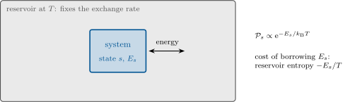
A system exchanging energy with a large reservoir at temperature $T$ occupies its microstate $s$ (energy $E_s$ ) with probability

\mathcal P_s = \frac{\eu^{-E_s/k_{\text{B}}T}}{Z} , \qquad Z = \sum_s \eu^{-E_s/k_{\text{B}}T}

( $\beta = 1/k_{\text{B}}T$ hereafter). $Z$ , the partition function, normalises the probabilities — and turns out to hold the entire thermodynamics of the system.

Proof. The system in state $s$ leaves the reservoir the energy $E - E_s$ : by the fundamental postulate applied to the whole, $\mathcal P_s \propto \Omega_{\text{res}}(E - E_s)$ . Expand the reservoir’s entropy, huge and smooth, to first order: $S_{\text{res}}(E - E_s) = S_{\text{res}}(E) - E_s\,\partial S_{\text{res}}/\partial E = S_{\text{res}}(E) - E_s/T$ by the definition of temperature. Hence $\Omega_{\text{res}} \propto \eu^{-E_s/k_{\text{B}}T}$ . (Higher orders die with the reservoir’s size.) ∎

Proposition 17.2 (The machine)

From $Z(T, V, N)$ :

\langle E\rangle = -\frac{\partial\ln Z}{\partial\beta} , \qquad F = -k_{\text{B}}T\ln Z , \qquad S = -\frac{\partial F}{\partial T} , \qquad P = -\frac{\partial F}{\partial V} ,

where $F = \langle E\rangle - TS$ is the free energy; and the heat capacity is a fluctuation:

C = \frac{\partial\langle E\rangle}{\partial T} = \frac{\langle E^2\rangle - \langle E\rangle^2} {k_{\text{B}}T^2} .

For independent, distinguishable subsystems $Z = z^N$ ; for $N$ identical particles in a common box, $Z = z^N/N!$ . At fixed $T$ and $V$ , equilibrium minimises $F$ : nature trades energy against entropy at the exchange rate $T$ — the single most useful principle in the physics of matter.

Partial proof. $-\partial_\beta\ln Z = \sum E_s\eu^{-\beta E_s}/Z = \langle E\rangle$ ; one more derivative gives $\langle E^2\rangle - \langle E\rangle^2$ , and the chain rule converts $\partial_\beta$ to $\partial_T$ . The identifications of $F$ , $S$ , $P$ follow by comparing $\dd(-k_{\text{B}}T\ln Z)$ with the thermodynamic $\dd F = -S\dd T - P\dd V$ ; factorisation is the exponential of a sum. The minimum principle: $F_{\text{system}}$ decreasing is $S_{\text{total}}$ increasing, since $\Delta S_{\text{res}} = -\Delta E_{\text{sys}}/T$ . ∎

The canonical setting: a small system borrowing energy from a vast reservoir. Each joule borrowed costs the reservoir 1/T of entropy — hence the exponential discount on energetic states. — The canonical setting: a small system borrowing energy from a vast reservoir. Each joule borrowed costs the reservoir $1/T$ of entropy — hence the exponential discount on energetic states.

17.2 First victories

Example 17.3 (Two levels, in two lines)

For levels $0, \epsilon$ : $z = 1 + \eu^{-\beta\epsilon}$ , giving $\langle E\rangle = N\epsilon/(\eu^{\beta\epsilon} + 1)$ — the result that cost the microcanonical route a page of Stirling (Exercise 16.8). The canonical formalism is the microcanonical one with the combinatorics pre-digested; the Schottky bump in $C(T)$ follows by one differentiation.

Example 17.4 (Einstein’s solid, and the death of Dulong–Petit)

Model a crystal as $3N$ quantum oscillators of frequency $\omega$ (Chapter 9). Per oscillator,

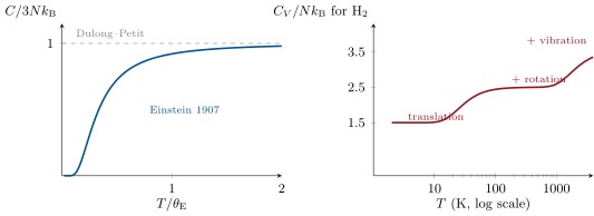
z = \sum_n\eu^{-\beta\hbar\omega(n + 1/2)} = \frac{1}{2\sinh(\beta\hbar\omega/2)} , \qquad \langle E\rangle = \frac{\hbar\omega}{2} + \frac{\hbar\omega}{\eu^{\beta\hbar\omega} - 1} .

At high $T$ : $\langle E\rangle \to k_{\text{B}}T$ per oscillator, $C \to 3Nk_{\text{B}}$ — the Dulong–Petit law of the Year 1 volume, explained. At low $T$ the quantum $\hbar\omega$ becomes unaffordable and $C$ collapses exponentially — as measured, and inexplicable classically. Einstein’s 1907 curve, one parameter per element, was the first application of quanta to ordinary matter; diamond, with stiff bonds and light atoms ( $\hbar\omega/k_{\text{B}} \approx 1300\,\mathrm{K}$ ), is still “frozen” at room temperature — the anomaly that had puzzled chemists for eighty years (Exercise 17.6).

Left: Einstein’s heat-capacity curve — classical equipartition regained at high T, quantum freezing below _ E = /k_ B. Right: hydrogen gas’s C_V climbs a staircase as rotation (near 85\, K) and then vibration (near 6000\, K, off scale) thaw: each motion joins equipartition only when k_ BT can pay its quantum. — Left: Einstein’s heat-capacity curve — classical equipartition regained at high $T$ , quantum freezing below $\theta_{\text{E}} = \hbar\omega/k_{\text{B}}$ . Right: hydrogen gas’s $C_V$ climbs a staircase as rotation (near $85\,\mathrm{K}$ ) and then vibration (near $6000\,\mathrm{K}$ , off scale) thaw: each motion joins equipartition only when $k_{\text{B}}T$ can pay its quantum.

Theorem 17.5 (Equipartition, with its licence)

Every coordinate or momentum entering the energy quadratically contributes, in the classical (high-temperature) regime,

\langle\epsilon\rangle = \tfrac12 k_{\text{B}}T

to the mean energy: $\tfrac32 k_{\text{B}}T$ for a monatomic gas atom, $\tfrac52$ for a rotating diatomic, $3k_{\text{B}}T$ for an oscillator. The licence expires when $k_{\text{B}}T$ falls below the mode’s level spacing: the mode freezes out and its contribution vanishes — the resolution of the nineteenth century’s heat-capacity scandals, drawn as the staircase above.

Partial proof. For $\epsilon = ax^2$ ,

\langle\epsilon\rangle = \frac{\int ax^2\,\eu^{-\beta ax^2}\dd x} {\int\eu^{-\beta ax^2}\dd x} = -\partial_\beta\ln\!\int\eu^{-\beta ax^2}\dd x = -\partial_\beta\ln\beta^{-1/2} = \frac{1}{2\beta} .

The freezing is Example 17.4’s computation, mode by mode. ∎

Example 17.6 (The gas, canonically)

One atom in a box: $z = V/\lambda_T^3$ (the state count of Proposition 7.5 weighted by Boltzmann); $N$ identical atoms: $Z = z^N/N!$ . Then $F = -Nk_{\text{B}}T[\ln(V/N\lambda_T^3) + 1]$ , and differentiation delivers $PV = Nk_{\text{B}}T$ , the Sackur–Tetrode entropy, and $\langle E\rangle = \tfrac32 Nk_{\text{B}}T$ — the whole ideal gas from one Gaussian integral. The Boltzmann factor applied to a molecule’s kinetic energy gives the Maxwell speed distribution of the Year 1 volume, now derived; applied to its potential energy $mgh$ it gives the exponential atmosphere — and, in a drop of water, Perrin’s ladder of grains (Problem 17.1).

Method 17.7 (Canonical craft)

(1) List the states and energies of one unit; compute $z$ . (2) Factorise: $Z = z^N$ (or $z^N/N!$ for identical particles sharing space); take $\ln$ early. (3) Differentiate: $\beta$ for energy, $T$ for entropy via $F$ , $V$ for pressure; a second derivative for $C$ and fluctuations. (4) Check both ends: high $T$ must reproduce equipartition, low $T$ must freeze with an $\eu^{-\Delta/k_{\text{B}}T}$ tail. (5) Competitions (folding, binding, alignment): write $F = E - TS$ for each alternative and let the smaller win — the crossover sits at $T \approx \Delta E/\Delta S$ .

17.3 Exercises

Exercise 17.1 ★

(a) Write the population ratio of two levels split by $\epsilon$ at temperature $T$ . (b) In a $2500\,\mathrm{K}$ flame, what fraction of sodium atoms sits in the $2.1\,\mathrm{eV}$ excited state of the D line (ground degeneracy 2, excited 6: population ratio $3\eu^{-\beta\epsilon}$ )? (c) Why does the flame nonetheless blaze yellow (how many atoms per cm $^3$ suffice)? (d) At what temperature would the excited fraction reach $10\%$ ?

Solution

Solution of Exercise 17.1.

(a) $\mathcal P_2/\mathcal P_1 = (g_2/g_1)\eu^{-\beta\epsilon}$ . (b) $\beta\epsilon = 2.1/(8.62\times10^{-5} \times 2500) = 9.7$ : fraction $3\eu^{-9.7} \approx 2 \times 10^{-4}$ . (c) A flame carries $\sim10^{15}$ sodium atoms per cm $^3$ : even $10^{-4}$ of them, cycling every few nanoseconds, pour out $10^{19}$ yellow photons per second — blinding. (d) $3\eu^{-\beta\epsilon} = 0.1$ : $T = \epsilon/(k_{\text{B}}\ln30) \approx 7200\,\mathrm{K}$ — a stellar photosphere, not a flame.

Exercise 17.2 ★

A three-level system: $0, \epsilon, 2\epsilon$ . (a) Write $z$ . (b) Compute $\langle E\rangle$ and check both temperature limits. (c) At what $T$ is the middle level maximally populated in absolute terms? (d) Show that no temperature, however high, makes a higher level more populated than a lower one — which chapter-16 concept would that require?

Solution

Solution of Exercise 17.2.

(a) $z = 1 + \eu^{-\beta\epsilon} + \eu^{-2\beta\epsilon}$ . (b) $\langle E\rangle = \epsilon(\eu^{-\beta\epsilon} + 2\eu^{-2\beta\epsilon})/z$ : $\to 0$ at low $T$ , $\to \epsilon$ (the mean level) at high. (c) $\mathcal P_1 = 1/(\eu^{\beta \epsilon} + 1 + \eu^{-\beta\epsilon})$ grows monotonically with $T$ , approaching its supremum $1/3$ only as $T \to \infty$ . (d) Boltzmann weights only decrease with energy at $T > 0$ ; a population inversion needs the negative temperatures of Example 16.8, unreachable by any reservoir.

Exercise 17.3 ★

The isothermal atmosphere. (a) Apply the Boltzmann factor to the potential energy $mgh$ and derive $n(h) = n_0\eu^{-mgh/k_{\text{B}} T}$ . (b) Compute the scale height for air ( $m = 4.8 \times 10^{-26}\,\mathrm{kg}$ ) at $288\,\mathrm{K}$ . (c) Everest’s summit pressure as a fraction of sea level. (d) Why is the real atmosphere’s fall-off close to but not exactly exponential (what did we hold constant that is not)?

Solution

Solution of Exercise 17.3.

(a) The Boltzmann factor on $E_p = mgh$ at uniform $T$ . (b) $h_0 = k_{\text{B}}T/mg = 8.4\,\mathrm{km}$ . (c) $\eu^{-8848/8440} \approx 0.35$ : one-third of an atmosphere — why summiteers carry oxygen. (d) The real atmosphere is not isothermal: temperature falls with height, so the profile bends away from a single exponential.

Exercise 17.4 ★

Equipartition bookkeeping. Count the quadratic terms and predict the molar $C_V$ of (a) argon; (b) N $_2$ at room temperature (rotation on, vibration frozen); (c) N $_2$ at $3000\,\mathrm{K}$ ; (d) a crystalline solid (Dulong–Petit). Where do the measured values $12.5$ , $20.8$ , $\approx26$ , $\approx25\,\mathrm{J}/(\mathrm{mol}\,\mathrm{K})$ agree, and what does each discrepancy teach?

Solution

Solution of Exercise 17.4.

(a) Three translations: $\tfrac32 R = 12.5\,\mathrm{J}/(\mathrm{mol}\,\mathrm{K})$ , agreed exactly. (b) Add two rotations: $\tfrac52 R = 20.8\,\mathrm{J}/(\mathrm{mol}\,\mathrm{K})$ , as measured: vibration is frozen. (c) $\tfrac72 R = 29.1\,\mathrm{J}/(\mathrm{mol}\,\mathrm{K})$ predicted; the measured $\approx26$ shows vibration only partly thawed ( $\theta_{\text{vib}} \approx 3400\,\mathrm{K}$ ). (d) $3R = 24.9\,\mathrm{J}/(\mathrm{mol}\,\mathrm{K})$ : Dulong–Petit, obeyed at room temperature by most metals and failed by diamond — the freezing story of Exercise 17.6.

Exercise 17.5 ★★

The quantum oscillator, canonically. (a) Sum the geometric series for $z$ . (b) Derive $\langle E\rangle$ and identify $\langle n\rangle = 1/(\eu^{\beta\hbar\omega} - 1)$ — the result of Exercise 9.6, now effortless. (c) Differentiate for $C(T)$ and verify the two limits. (d) Why is $\langle n\rangle$ ’s form about to become famous (Chapter 20)?

Solution

Solution of Exercise 17.5.

(a) $z = \eu^{-\beta\hbar\omega/2}/(1 - \eu^{-\beta\hbar\omega})$ . (b) $\langle E\rangle = -\partial_\beta\ln z$ gives the stated form with $\langle n\rangle = 1/(\eu^{\beta\hbar\omega} - 1)$ . (c) $C \to k_{\text{B}}$ at high $T$ ; $C \approx k_{\text{B}}(\beta \hbar\omega)^2\eu^{-\beta\hbar\omega} \to 0$ at low. (d) With $\hbar\omega$ the energy of a light quantum, $\langle n\rangle$ is the thermal photon number per mode: Planck’s law is one chapter away.

Exercise 17.6 ★★

Einstein versus the data. (a) From the figure’s formula, at what $T/\theta_{\text{E}}$ has $C$ fallen to half of Dulong–Petit? (b) Diamond: $\theta_{\text{E}} \approx 1300\,\mathrm{K}$ — compute $C/3Nk_{\text{B}}$ at $300\,\mathrm{K}$ and explain the nineteenth century’s “anomaly of diamond”. (c) Lead: $\theta_{\text{E}} \approx 90\,\mathrm{K}$ — why was lead always “well-behaved”? (d) Measurements at very low $T$ show $C \propto T^3$ , not exponential: which of Einstein’s assumptions fails (all oscillators one frequency), and who repaired it (Chapter 20)?

Solution

Solution of Exercise 17.6.

(a) Numerically, $C = \tfrac12 \times 3Nk_{\text{B}}$ near $T/\theta_{\text{E}} \approx 0.34$ . (b) $\theta_{\text{E}}/T = 4.3$ : $C/3Nk_{\text{B}} = 4.3^2\eu^{-4.3}/(1 - \eu^{-4.3})^2 \approx 0.26$ — diamond at room temperature has barely a quarter of the classical heat capacity: the “anomaly” is quantum freezing in plain sight. (c) $\theta_{\text{E}} = 90\,\mathrm{K}$ puts lead deep in the classical regime at $300\,\mathrm{K}$ . (d) The single-frequency assumption: real solids have a spectrum of modes down to long-wavelength sound, whose cheap quanta give the $T^3$ law — Debye’s repair, in Chapter 20.

Exercise 17.7 ★★

Maxwell’s tail and the missing hydrogen. (a) From the Boltzmann factor on kinetic energy, write the speed distribution and locate the most probable speed for N $_2$ and H $_2$ at $288\,\mathrm{K}$ . (b) Earth’s escape speed is $11.2\,\mathrm{km}/\mathrm{s}$ : compute $mv_{\text{esc}}^2/2k_{\text{B}}T$ for both gases. (c) The escaping fraction goes as $\eu^{-mv_{\text{esc}}^2/2k_{\text{B}}T}$ : compare the two exponents and conclude which gas leaks over geological time. (d) Connect to the observed composition of Earth’s (no free H $_2$ ) versus Jupiter’s (mostly H $_2$ ) atmospheres — what two parameters flip the verdict?

Solution

Solution of Exercise 17.7.

(a) $f(v) \propto v^2\eu^{-mv^2/2k_{\text{B}}T}$ : $v_{\text{p}} = \sqrt{2k_{\text{B}}T/m}$ : $413\,\mathrm{m}/\mathrm{s}$ for N $_2$ , $1540\,\mathrm{m}/\mathrm{s}$ for H $_2$ . (b) $mv_{\text{esc}}^2/2k_{\text{B}}T \approx 730$ for N $_2$ , $52$ for H $_2$ . (c) $\eu^{-730}$ is never; $\eu^{-52} \sim 10^{-23}$ per residence time is slow — but the hot upper atmosphere ( $\sim1000\,\mathrm{K}$ ) softens the hydrogen exponent to $\sim15$ : hydrogen bleeds away over geological time, nitrogen stays. (d) Escape speed and exospheric temperature: Jupiter’s $60\,\mathrm{km}/\mathrm{s}$ well makes even hydrogen’s exponent astronomical — gas giants keep what small warm worlds lose.

Exercise 17.8 ★★

Fluctuations meet response. (a) Prove $C = (\langle E^2\rangle - \langle E\rangle^2)/k_{\text{B}}T^2$ from two derivatives of $\ln Z$ . (b) Verify it explicitly on the two-level system. (c) For $N$ independent units, show the relative energy fluctuation falls as $1/\sqrt N$ . (d) State the moral: what a system’s willingness to absorb heat (a response) has to do with how much its energy jitters (a fluctuation) — statistical physics’ recurring bargain.

Solution

Solution of Exercise 17.8.

(a) $\partial_\beta^2\ln Z = \langle E^2\rangle - \langle E\rangle^2$ , and $C = \partial_T\langle E\rangle = -k_{\text{B}}\beta^2\partial_\beta\langle E\rangle$ . (b) Both sides give $Nk_{\text{B}}(\beta\epsilon)^2\eu^{\beta\epsilon}/( \eu^{\beta\epsilon} + 1)^2$ . (c) $\langle E\rangle \propto N$ , $\Delta E \propto \sqrt N$ . (d) How strongly a system responds to heating equals how much its energy spontaneously jitters — response and fluctuation are two readings of the same second derivative, a pattern (fluctuation–dissipation) that recurs throughout physics.

Exercise 17.9 ★★

Boltzmann in the chemistry lab. Reaction rates carry the factor $\eu^{-E_a/k_{\text{B}}T}$ (crossing an activation barrier $E_a$ — Arrhenius). (a) Show the rule of thumb “rate doubles every $10\,\mathrm{K}$ near room temperature” corresponds to $E_a \approx 0.55\,\mathrm{eV}$ . (b) By what factor does that reaction slow in a refrigerator ( $5\,{}^{\circ}\mathrm{C}$ )? (c) Cooking an egg at altitude: water boils at $93\,{}^{\circ}\mathrm{C}$ on a $2000\,\mathrm{m}$ pass — estimate the extra cooking time. (d) Why does a barrier tail, not the mean energy, rule chemistry (which molecules react)?

Solution

Solution of Exercise 17.9.

(a) $\ln2 = E_a\,\Delta T/k_{\text{B}}T^2$ with $\Delta T = 10\,\mathrm{K}$ , $T = 298\,\mathrm{K}$ : $E_a = 0.693\,k_{\text{B}}T^2/10 \approx 0.55\,\mathrm{eV}$ . (b) From $298$ to $278\,\mathrm{K}$ : factor $\eu^{E_a(1/278 - 1/298)/k_{\text{B}}} \approx 4.4$ slower — why refrigerators preserve food. (c) $373 \to 366\,\mathrm{K}$ : rate falls by $\approx1.4$ : the eleven-minute egg needs a quarter of an hour. (d) Reactions are won by the exponential tail of molecules above the barrier: shift the temperature slightly and the tail’s population shifts enormously — the mean hardly matters.

Exercise 17.10 ★★★

Two-state folding. A biomolecule is folded (energy $0$ , one configuration) or unfolded (energy $\Delta E > 0$ , $\Omega_u = \eu^{\Delta S/k_{\text{B}}}$ configurations). (a) Write the folded fraction versus $T$ . (b) Show the “melting” midpoint is $T_{\text{m}} = \Delta E/\Delta S$ and interpret as an $F = E - TS$ tie. (c) With $\Delta E = 3.0\,\mathrm{eV}$ and $\Delta S = 100\,k_{\text{B}}$ (a small protein’s cooperative unit): compute $T_{\text{m}}$ and the width of the transition. (d) Why does cooperativity (many contacts breaking together, large $\Delta E$ and $\Delta S$ ) sharpen melting — and how do DNA thermal-cycling machines (PCR) exploit exactly this?

Solution

Solution of Exercise 17.10.

(a) $f_{\text{folded}} = 1/(1 + \eu^{-\beta(\Delta E - T\Delta S)})$ with the unfolded state’s entropy folded into its free energy. (b) At $T_{\text{m}} = \Delta E/\Delta S$ the two free energies tie: half and half. (c) $T_{\text{m}} = 4.8 \times 10^{-19}/1.38 \times 10^{-21} = 348\,\mathrm{K}$ ( $75\,{}^{\circ}\mathrm{C}$ ); width $\delta T \sim k_{\text{B}}T_{\text{m}}^2/\Delta E \approx 3.5\,\mathrm{K}$ . (d) Cooperativity multiplies both $\Delta E$ and $\Delta S$ by the number of contacts breaking together, keeping $T_{\text{m}}$ but shrinking the width $\propto 1/\Delta E$ : DNA strands separate over a couple of kelvin, which is what lets a PCR machine cycle cleanly between “melted” and “annealed”.

Exercise 17.11 ★★★

Paramagnetism and magnetic cooling. $N$ spins $\tfrac12$ of moment $\mu$ in field $B$ . (a) Show $M = N\mu\tanh(\mu B/k_{\text{B}}T)$ and expand to Curie’s law $M \approx N\mu^2B/k_{\text{B}}T$ . (b) Evaluate the alignment $\mu B/k_{\text{B}}T$ for electron moments at $B = 1\,\mathrm{T}$ , $T = 300\,\mathrm{K}$ and at $1\,\mathrm{K}$ . (c) Adiabatic demagnetisation: magnetise at $1\,\mathrm{K}$ , isolate, reduce $B$ tenfold — show constant entropy means constant $\mu B/k_{\text{B}}T$ , so $T$ drops tenfold. (d) What sets the floor of this refrigerator (interactions between the spins — estimate the dipolar scale $\mu_0\mu^2/4\pi a^3$ for $a = 0.5\,\mathrm{nm}$ , in temperature units)?

Solution

Solution of Exercise 17.11.

(a) $z = 2\cosh(\beta\mu B)$ ; $M = N\mu\tanh(\beta\mu B) \approx N\mu^2B/k_{\text{B}}T$ for small argument: Curie’s $1/T$ . (b) $\mu_{\text{B}}B/k_{\text{B}}T$ : $2.2 \times 10^{-3}$ at $300\,\mathrm{K}$ ; $0.67$ at $1\,\mathrm{K}$ — from indifferent to strongly aligned. (c) $S$ depends on $\mu B/k_{\text{B}}T$ alone; lowering $B$ at fixed entropy drags $T$ down proportionally: $1\,\mathrm{K} \to 0.1\,\mathrm{K}$ . (d) When $k_{\text{B}}T$ reaches the spin–spin energy the entropy is no longer field-controlled: $\mu_0\mu_{\text{B}}^2/4\pi a^3 \approx 7 \times 10^{-26}\,\mathrm{J} \sim 5\,\mathrm{mK}$ — the classic floor (nuclear moments, a thousand times weaker, push it to microkelvins).

Exercise 17.12 ★★★

The rotational staircase, quantitatively. A diatomic’s rotational levels are $E_J = BJ(J+1)$ , degeneracy $2J + 1$ (Chapter 10). (a) Write $z_{\text{rot}}$ and show that for $k_{\text{B}}T \gg B$ the sum becomes the integral $k_{\text{B}}T/B$ : equipartition’s $k_{\text{B}}$ in $C_V$ regained. (b) Define $\theta_{\text{rot}} = B/k_{\text{B}}$ and evaluate for H $_2$ ( $B = 7.5\,\mathrm{meV}$ ) and N $_2$ ( $B = 0.25\,\mathrm{meV}$ ): which gas shows the rotational step at accessible temperatures? (c) Sketch hydrogen’s full $C_V(T)$ staircase with its three plateaus and two risers, placing numbers on both. (d) The measured low- $T$ behaviour of H $_2$ is further complicated by the 3:1 ortho–para mixture of Exercise 14.8: state in one sentence how nuclear spin statistics reaches into a gas’s heat capacity.

Solution

Solution of Exercise 17.12.

(a) $z_{\text{rot}} = \sum_J(2J+1)\eu^{-\beta BJ(J+1)} \to \int(2J+1)\eu^{-\beta BJ(J+1)}\dd J = k_{\text{B}}T/B$ : then $\langle E\rangle = k_{\text{B}}T$ and $C_{\text{rot}} = k_{\text{B}}$ . (b) H $_2$ : $\theta_{\text{rot}} = 87\,\mathrm{K}$ — the step sits in the laboratory range; N $_2$ : $2.9\,\mathrm{K}$ , frozen out only near liquid helium, so nitrogen always shows $\tfrac52 R$ . (c) Plateaus $\tfrac32 R$ (below $\sim50\,\mathrm{K}$ ), $\tfrac52 R$ (from $\sim200$ to $\sim1000\,\mathrm{K}$ ), rising toward $\tfrac72 R$ near $\theta_{\text{vib}} \approx 6000\,\mathrm{K}$ . (d) Odd and even $J$ belong to different nuclear spin species that interconvert slowly, so cold hydrogen’s $C_V$ depends on its ortho–para history — nuclear statistics audited by a calorimeter.

17.4 Problem: Counting Avogadro in a drop of water

Problem 17.1

Weekend problem — Perrin’s grains and the reality of atoms

In 1908 Jean Perrin suspended microscopic resin grains in water, let them settle, and counted them layer by layer under a microscope. The exponential ladder he found was the Boltzmann factor made visible — and from its scale height he extracted Avogadro’s number, convincing the last sceptics that atoms exist. Nobel Prize, 1926. Data: gamboge grains of radius $r = 0.212\,\text{µ}\mathrm{m}$ , density $\rho_{\text{g}} = 1207\,\mathrm{kg}/\mathrm{m}^{3}$ ; water $\rho_{\text{w}} = 999\,\mathrm{kg}/\mathrm{m}^{3}$ ; $T = 293\,\mathrm{K}$ ; $g = 9.81\,\mathrm{m}/\mathrm{s}^{2}$ .

Part I — The visible Boltzmann factor.

A grain in water feels gravity minus buoyancy: compute its effective mass $m' = \tfrac43\pi r^3(\rho_{\text{g}} - \rho_{\text{w}})$ and weight.
Write the equilibrium concentration profile $n(h)$ from the Boltzmann factor.
Compute the scale height $h_0 = k_{\text{B}}T/m'g$ with the modern $k_{\text{B}}$ .
Why must the grains be so precisely mono-sized (how does $h_0$ depend on $r$ )?
Compare $h_0$ with the same formula for air molecules: why is the grains’ atmosphere micrometres tall while the air’s is kilometres?
Perrin counted (in one run) relative concentrations $100 : 55 : 30 : 17$ at four equally spaced depths $30\,\text{µ}\mathrm{m}$ apart: check that this is an exponential ladder and extract its $h_0$ .

Part II — Weighing the invisible.

Invert: from the measured $h_0$ of item 6 and the known $m'g$ , extract $k_{\text{B}}$ .
The gas constant $R = 8.314\,\mathrm{J}/(\mathrm{mol}\,\mathrm{K})$ was known from macroscopic chemistry: combine with your $k_{\text{B}}$ to obtain Avogadro’s number $N_{\text{A}} = R/k_{\text{B}}$ .
Perrin’s runs gave $N_{\text{A}}$ between $5.5$ and $7.2 \times 10^{23}$ : compare with the modern $6.022 \times 10^{23}$ and comment on the achievement given his microscope and stopwatch.
From $N_{\text{A}}$ , compute the mass of a single hydrogen atom — the number the atomists had wanted for a century.
Explain the logical structure: which macroscopic measurements ( $R$ ; grain size and density; the ladder) combine to weigh one atom, with no atom ever seen?
Why do the grains — $10^{10}$ atomic masses each — obey the same Boltzmann statistics as molecules (what in the derivation of Theorem 17.1 cares about size)?

Part III — The jitter that seals it.

The same grains jitter: Einstein’s 1905 formula for Brownian motion gives $\langle x^2\rangle = 2Dt$ with $D = k_{\text{B}}T/6\pi\eta r$ (water: $\eta = 10^{-3}\,\mathrm{Pa}\,\mathrm{s}$ ). Compute $D$ for Perrin’s grains.
How far does a grain wander in one minute? Could Perrin measure it with a micrometer eyepiece and a stopwatch?
Perrin verified $\langle x^2\rangle \propto t$ and extracted $k_{\text{B}}$ again, independently: why did two unrelated routes (a static ladder; a dynamic jitter) to one number carry such evidential weight?
The jitter is equipartition applied to the grain: each velocity component carries $\tfrac12 k_{\text{B}}T$ . Estimate the grain’s r.m.s. thermal speed ( $m \approx 4.8 \times 10^{-17}\,\mathrm{kg}$ ).
Why is that speed never seen directly (what interrupts the free flight after nanometres), and what is seen instead?
State which two chapters of this book meet in the observation: the mechanics of drag (Year 2 volume, viscosity) and the statistics of this chapter.

Part IV — What was settled.

Ostwald and Mach had held atoms to be bookkeeping fictions: state in one sentence why a counted $N_{\text{A}}$ from grain ladders ended that position.
List three other 1900s routes that converged on the same $N_{\text{A}}$ (blue of the sky, Exercise 16.12; electrolysis plus the electron charge; radioactivity’s helium production) — why did convergence matter more than any single value?
Perrin’s ladder is an equilibrium between which two currencies of this chapter (energy pulling down, entropy spreading up), priced at which rate?
Modern uses of the same physics: analytical ultracentrifuges spin proteins at $10^5g$ to compress their “atmospheres” into measurable ladders — show that multiplying $g$ by $10^5$ divides $h_0$ by the same factor, and estimate $h_0$ for a protein of effective mass $10^{-22}\,\mathrm{kg}$ at $10^5g$ , $293\,\mathrm{K}$ .
Doubling the grain radius divides $h_0$ by eight: bracket the practical window of grain sizes between “ladder too tall to see a gradient” and “ladder thinner than one grain” for a microscope field $100\,\text{µ}\mathrm{m}$ deep.
Since 2019 the SI defines $k_{\text{B}}$ and $N_{\text{A}}$ exactly: state what an exact Perrin-style experiment measures today (a consistency check, or a calibration of the apparatus and grains) — and why the physics is unchanged.
Summarise the named result: a $0.2\,\text{µ}\mathrm{m}$ grain’s concentration halves every $\sim35\,\text{µ}\mathrm{m}$ of height; read with $n(h) = n_0\eu^{-m'gh/k_{\text{B}}T}$ , that ladder yielded $N_{\text{A}} \approx 6 \times 10^{23}$ — atoms counted, not conjectured, in a drop of water on a microscope stage.

Solution

Solution of Problem 17.1.

1. $V = \tfrac43\pi r^3 = 4.0 \times 10^{-20}\,\mathrm{m}^{3}$ : $m' = V \Delta\rho = 8.3 \times 10^{-18}\,\mathrm{kg}$ , weight $m'g = 8.1 \times 10^{-17}\,\mathrm{N}$ . 2. $n(h) = n_0\,\eu^{-m'gh/k_{\text{B}}T}$ : the barometric law, shrunk to a microscope slide. 3. $h_0 = k_{\text{B}}T/m'g = 4.04 \times 10^{-21}/8.1 \times 10^{-17} \approx 50\,\text{µ}\mathrm{m}$ . 4. $h_0 \propto 1/r^3$ : a $10\%$ spread in radius is a $30\%$ spread in scale height — polydisperse grains smear the ladder into mush. Perrin fractionated for months by repeated centrifugation. 5. Same formula, masses $10^{10}$ apart: the grain “atmosphere” is $10^{10}$ times shallower — kilometres shrink to tens of micrometres, which is precisely what makes it observable whole under a microscope. 6. Successive ratios $0.55$ , $0.55$ , $0.57$ : constant within counting error — exponential. $h_0 = 30\,\text{µ}\mathrm{m}/\ln(100/55) \approx 50\,\text{µ}\mathrm{m}$ . 7. $k_{\text{B}} = m'g\,h_0/T = 8.1 \times 10^{-17} \times 5.0 \times 10^{-5}/293 \approx 1.4 \times 10^{-23}\,\mathrm{J}/\mathrm{K}$ . 8. $N_{\text{A}} = R/k_{\text{B}} \approx 6.0 \times 10^{23}\,\mathrm{mol}^{-1}$ . 9. Within a few per cent here (with idealised data); Perrin’s real runs scattered by $\pm15\%$ around the modern value — astonishing for hand-counted grains, and utterly decisive for the order of magnitude. 10. $m_{\text{H}} = 10^{-3}\,\mathrm{kg}/\mathrm{mol}/N_{\text{A}} = 1.7 \times 10^{-27}\,\mathrm{kg}$ . 11. Macroscopic chemistry supplies $R$ ; light microscopy and weighing supply $m'$ ; counting supplies the ladder: three tabletop measurements triangulate the mass of an atom no one can see. 12. Nothing: the derivation used only “system exchanging energy with a reservoir” — Boltzmann’s factor is size-blind, which is exactly what Perrin verified. 13. $D = k_{\text{B}}T/6\pi\eta r = 4.04 \times 10^{-21}/4.0 \times 10^{-9} \approx 10^{-12}\,\mathrm{m}^{2}/\mathrm{s}$ . 14. $\sqrt{2Dt} = \sqrt{1.2 \times 10^{-10}} \approx 11\,\text{µ}\mathrm{m}$ per minute: comfortably measurable with an eyepiece graticule and patience. 15. Two independent phenomena, two independent formulas, one number: agreement of the static ladder and the dynamic jitter left no niche for coincidence — the molecular hypothesis predicted both. 16. $\sqrt{k_{\text{B}}T/m} = \sqrt{4.04 \times 10^{-21}/ 4.8 \times 10^{-17}} \approx 9\,\mathrm{mm}/\mathrm{s}$ per component. 17. The grain is struck $10^{19}$ times per second and forgets its velocity within nanometres: the ballistic flight is unobservable, and what the eye sees is its integral — the diffusive random walk. 18. Stokes drag (the viscosity of the Year 2 volume’s fluids) supplies the $6\pi\eta r$ ; the canonical ensemble supplies the $k_{\text{B}}T$ : Einstein’s $D$ is their quotient, mechanics and statistics in one fraction. 19. A fiction cannot be counted: once $N_{\text{A}}$ is the ratio of two measured numbers, with error bars, atoms are objects of experiment — Ostwald conceded in print in 1909. 20. Sky-blue scattering, electrolysis with the measured electron charge, helium accumulated from radium: four unrelated physical channels converging on one $6\times10^{23}$ made the number a property of nature rather than of any theory. 21. Gravitational energy pulling the grains down, configurational entropy spreading them up, traded at the rate $T$ : the ladder is the minimum of $F = E - TS$ . 22. $h_0 \propto 1/g$ : at $10^5g$ , $h_0 = k_{\text{B}}T/(m'\times10^5g) = 4.04 \times 10^{-21}/ 9.8 \times 10^{-17} \approx 40\,\text{µ}\mathrm{m}$ for the protein — sedimentation equilibrium, Perrin’s experiment run daily in biochemistry departments. 23. From “too tall” ( $h_0 \gg$ field depth: no visible gradient) to “too thin” ( $h_0 \lesssim r$ ): usable radii span roughly $0.1$ – $0.5\,\text{µ}\mathrm{m}$ — Perrin’s choice was not luck but design. 24. With $k_{\text{B}}$ now exact by definition, the same experiment calibrates the grains (their size or density) or audits the setup: the physics — Boltzmann’s ladder — is untouched; only which quantity counts as unknown has moved. 25. A $0.2\,\text{µ}\mathrm{m}$ grain’s population halves every $\sim35\,\text{µ}\mathrm{m}$ ; read through $n_0\eu^{-m'gh/k_{\text{B}} T}$ , the ladder returned $N_{\text{A}} \approx 6 \times 10^{23}$ : Avogadro’s number counted grain by grain — and the atomic debate closed on a microscope stage.