University Physics — Year 3 · Bachelor Year 3

7The Schrödinger Equation in Three Dimensions

The screen of a modern television glows with crystals so small that their size sets their colour: a cadmium-selenide grain four nanometres across shines red, the same substance at two nanometres shines blue-green. Nothing in the chemistry differs — only the size of the box confining the electrons. The Year 2 volume ended with quantum mechanics in one dimension: wave functions on a line, wells, barriers and tunnelling. But electrons live in three dimensions, and the step from the line to space brings genuinely new physics: probability flows as a current through space, energies of a box pile up with degeneracies that betray its symmetry, states must be counted — the count that will later run all of statistical physics — and spherical problems reduce, at their simplest, to a disguised one-dimensional equation on the radius. This chapter makes those steps, and its centrepieces are a television’s quantum dot and the lightest nucleus in nature.

7.1 Wave functions in space

Definition 7.1 (Wave function and probability in three dimensions)

The state of a particle is a complex field $\psi(\vect r, t)$ with Born’s rule

\dd\mathcal P = |\psi(\vect r, t)|^2\,\dd^3r , \qquad \int|\psi|^2\,\dd^3r = 1 ,

and its evolution is the Schrödinger equation with the Laplacian in place of the second derivative:

\iu\hbar\,\frac{\partial\psi}{\partial t} = -\frac{\hbar^2}{2m}\,\Delta\psi + V(\vect r)\,\psi , \qquad \Delta = \frac{\partial^2}{\partial x^2} + \frac{\partial^2}{\partial y^2} + \frac{\partial^2}{\partial z^2} .

Everything the Year 2 volume established survives verbatim: linearity and superposition, stationary states $\varphi(\vect r)\,\eu^{-\iu Et/\hbar}$ with $-\tfrac{\hbar^2}{2m}\Delta\varphi + V\varphi = E\varphi$ , and the momentum operator, now the gradient $\hat{\vect p} = -\iu\hbar\vect\nabla$ .

Proposition 7.2 (Probability flows: the current)

The density $\rho = |\psi|^2$ obeys a continuity equation,

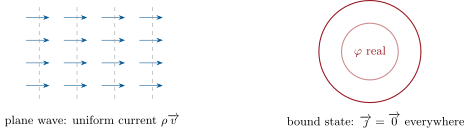
\frac{\partial\rho}{\partial t} + \operatorname{div}\vect\jmath = 0 , \qquad \vect\jmath = \frac{\hbar}{m}\, \operatorname{Im}\big(\psi^*\vect\nabla\psi\big) :

probability is locally conserved, transported by the current $\vect\jmath$ — for a plane wave $A\eu^{\iu\vect k\cdot\vect r}$ , $\vect\jmath = |A|^2\hbar\vect k/m = \rho\vect v$ , a uniform flow; for any real-valued $\varphi$ , $\vect\jmath = \vect 0$ : bound stationary states carry no net flow.

Proof. As in one dimension: $\partial_t(\psi^*\psi)$ from the equation and its conjugate; the potential terms cancel, and $(\iu\hbar/2m) (\psi^*\Delta\psi - \psi\Delta\psi^*) = -\operatorname{div}\big[(\hbar/m)\operatorname{Im}(\psi^*\vect\nabla \psi)\big]$ by the product rule for the divergence. ∎

The probability current: a travelling wave transports its density like a fluid; a real (bound, stationary) wave function stands still — the atom’s electron cloud does not circulate unless the state is complex.

7.2 Boxes, degeneracy, and the counting of states

Theorem 7.3 (Separation of variables)

If the potential splits as $V = V_1(x) + V_2(y) + V_3(z)$ , the stationary states can be taken as products $\varphi(\vect r) = \varphi_1(x)\,\varphi_2(y)\,\varphi_3(z)$ , where each factor solves its own one-dimensional problem, and the energies add: $E = E_1 + E_2 + E_3$ . Three dimensions, in such cases, is one dimension three times.

Proof. Insert the product into the stationary equation and divide by $\varphi$ : the sum of three single-variable expressions equals the constant $E$ , so each is separately constant. That every state is a superposition of such products is the completeness of the 1D solutions, admitted. ∎

Proposition 7.4 (The cubic box and its degeneracies)

In a box of side $a$ with impenetrable walls, the states are indexed by three positive integers,

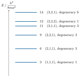
\varphi_{n_1n_2n_3} \propto \sin\frac{n_1\pi x}{a}\sin\frac{n_2\pi y}{a}\sin\frac{n_3\pi z}{a} , \qquad E = \frac{h^2}{8ma^2}\,(n_1^2 + n_2^2 + n_3^2) .

Distinct states now share energies: the level $(2,1,1)$ comes in three copies, $(1,2,1)$ and $(1,1,2)$ being physically distinct states of the same $E$ . Such degeneracy is the signature of symmetry — here, the interchangeability of the box’s three axes; squash the box slightly and the triplet splits.

Proof. Separation with three infinite wells of the Year 2 volume; the energies add. ∎

The lowest levels of the cubic box: energies in units of h2/8ma2 with their quantum numbers. Permutations of unequal n_i give degenerate triplets and sextets — the fingerprint of cubic symmetry. — The lowest levels of the cubic box: energies in units of $h^2/8ma^2$ with their quantum numbers. Permutations of unequal $n_i$ give degenerate triplets and sextets — the fingerprint of cubic symmetry.

Proposition 7.5 (Counting states)

The number of box states with energy below $E$ is, for $E$ large,

N(E) \approx \frac{V}{6\pi^2}\Big(\frac{2mE}{\hbar^2}\Big)^{3/2} , \qquad V = a^3 :

proportional to the volume and to $E^{3/2}$ . Equivalently, phase space holds one quantum state per volume $h^3$ — the Bohr–Sommerfeld cell of Chapter 2, now derived. This single count is the raw material of the statistical physics and the solid-state physics later in this volume: electrons in metals, photons in cavities, the glow of hot bodies all begin here.

Proof. States are lattice points $(n_1, n_2, n_3)$ in the positive octant; $E \le E_{\max}$ keeps those inside the sphere of radius $R = \sqrt{8ma^2E/h^2}$ . For large $R$ , the count is the octant volume $\tfrac18\cdot\tfrac43\pi R^3$ ; substitute. (Phase-space version: $N = \tfrac{V\cdot\frac43\pi p^3}{h^3}$ with $p = \sqrt{2mE}$ — the same number.) ∎

Example 7.6 (A metal, first estimate)

Copper offers roughly one mobile electron per atom, $n = 8.5 \times 10^{28}\,\mathrm{m}^{-3}$ . Filling the box states two electrons each (spin, Chapter 12) up to the energy that accommodates them all gives, inverting the count, $E_{\text{F}} \approx 7\,\mathrm{eV}$ — an enormous energy compared with thermal agitation ( $k_{\text{B}}T \approx 25\,\mathrm{meV}$ ): even at room temperature a metal’s electrons are a profoundly quantum crowd. The full story is Chapter 24.

Example 7.7 (The isotropic oscillator)

For $V = \tfrac12 m\omega^2r^2 = \tfrac12 m\omega^2(x^2 + y^2 + z^2)$ , separation gives $E = (n_x + n_y + n_z + \tfrac32)\hbar\omega$ : levels $\tfrac32, \tfrac52, \tfrac72\hbar\omega\ldots$ with degeneracies $1, 3, 6, 10, \dots$ — growing, unlike the box’s irregular pattern, with perfect regularity. Extra degeneracy beyond what axis-permutation explains signals a larger hidden symmetry; the hydrogen atom will repeat the trick spectacularly. Filled with spin-paired particles, these oscillator shells hold $2, 8, 20, \dots$ — the first approximation to the “magic numbers” of nuclear physics (Chapter 25).

7.3 Spherical problems: the s-wave trick

Proposition 7.8 (Spherically symmetric states)

For a central potential $V(r)$ , seek states depending on $r$ alone (the s states; the general case, with angular structure, waits for Chapter 10). Writing $\varphi(r) = u(r)/r$ , the function $u$ obeys

-\frac{\hbar^2}{2m}\,u'' + V(r)\,u = E\,u , \qquad u(0) = 0 :

exactly the one-dimensional Schrödinger equation on a half-line, with a wall at the origin. Every 1D tool of the Year 2 volume — wells, matching, tunnelling — applies verbatim to spherical problems, at the price of one substitution.

Proof. For $\varphi(r)$ , the Laplacian reduces to $\Delta\varphi = \tfrac1r(r\varphi)'' = u''/r$ ; insert and multiply by $r$ . The condition $u(0) = 0$ keeps $\varphi = u/r$ finite at the origin; normalisation is $\int_0^\infty|u|^2\dd r$ times $4\pi$ — $u$ is a genuine 1D wave function. ∎

Example 7.9 (The deuteron: barely a nucleus)

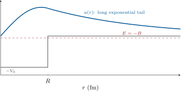
The deuteron — one proton, one neutron — is the simplest nucleus: binding energy $B = 2.2\,\mathrm{MeV}$ , tiny beside nuclear scales. As a model, put the relative motion (reduced mass $m_{\text{p}}/2$ ) in a spherical well of range $R = 2.1\,\mathrm{fm}$ and depth $V_0$ : the $u$ equation is the finite 1D well. Matching inside and outside solutions demands a minimum depth $V_0 > \pi^2\hbar^2/8\mu R^2 \approx 23\,\mathrm{MeV}$ for any bound state, and reproducing $B = 2.2\,\mathrm{MeV}$ requires $V_0 \approx 35\,\mathrm{MeV}$ (Exercise 7.10): the strong force binds the deuteron by only ten per cent of margin. The wave function leaks far outside the well — the nucleon pair spends most of its time beyond the force’s reach — and there is no second bound state: nature’s second-simplest nucleus, helium, needs a third nucleon.

The deuteron’s radial wave function u(r) in the spherical-well model: barely one quarter-oscillation fits inside the well, and the state survives on a tail reaching far beyond the range of the force — a nucleus bound by 2.2\, MeV in a well 35\, MeV deep. — The deuteron’s radial wave function $u(r)$ in the spherical-well model: barely one quarter-oscillation fits inside the well, and the state survives on a tail reaching far beyond the range of the force — a nucleus bound by $2.2\,\mathrm{MeV}$ in a well $35\,\mathrm{MeV}$ deep.

Method 7.10 (Three-dimensional problems)

(1) Additive potential ( $V_1 + V_2 + V_3$ )? Separate; energies add; collect degeneracies by symmetry. (2) Central potential, spherical state? Substitute $\varphi = u/r$ and reuse every 1D result with $u(0) = 0$ . (3) To count states, think in $\vect n$ space or in phase space at one state per $h^3$ (per spin state). (4) Currents: compute $\vect\jmath$ when a flow or a flux matters; remember real wave function $=$ no current. (5) Estimates first: confinement energy $\sim h^2/8mL^2$ per direction decides scales from quantum dots to nuclei before any equation is solved.

Quantum dots under ultraviolet light: the same semiconductor, in ever-smaller crystals, glows from red to blue. The colour is set by the particle-in-a-box energies of this chapter — confinement you can see.

7.4 Exercises

Exercise 7.1 ★

The Gaussian state $\psi(\vect r) = A\,\eu^{-r^2/4\sigma^2}$ . (a) Normalise ( $\int_0^\infty x^2\eu^{-x^2}\dd x = \sqrt\pi/4$ ). (b) Compute $\langle r^2\rangle$ and $\Delta x$ (isotropy helps). (c) What is $\vect\jmath$ for this state, and why? (d) Multiply by $\eu^{\iu\vect k_0\cdot\vect r}$ : what are now $\langle\vect p\rangle$ and $\vect\jmath$ ?

Solution

Solution of Exercise 7.1.

(a) $\int|\psi|^2\dd^3r = |A|^2\,4\pi\int_0^\infty r^2\eu^{-r^2/2 \sigma^2}\dd r = |A|^2(2\pi\sigma^2)^{3/2}$ : $A = (2\pi\sigma^2)^{ -3/4}$ . (b) By isotropy $\langle r^2\rangle = 3\langle x^2\rangle = 3\sigma^2$ , so $\Delta x = \sigma$ . (c) $\vect\jmath = \vect 0$ : the wave function is real. (d) $\langle\vect p\rangle = \hbar\vect k_0$ and $\vect\jmath = \rho\,\hbar\vect k_0/m$ : the same cloud, now drifting.

Exercise 7.2 ★

For the cubic box, list all levels up to $E = 15$ (units of $h^2/8ma^2$ ) with their degeneracies. Then show that the level $27$ is degenerate beyond permutations: find its two families of quantum numbers, and say why such “accidental” degeneracy does not follow from cubic symmetry.

Solution

Solution of Exercise 7.2.

$3\,(1)$ , $6\,(3)$ , $9\,(3)$ , $11\,(3)$ , $12\,(1)$ , $14\,(6)$ — then nothing until $17$ . Level $27$ : $(3,3,3)$ and the permutations of $(5,1,1)$ — four states, since $27 = 9+9+9 = 25+1+1$ . Cubic symmetry only permutes axes, and no permutation links $(3,3,3)$ to $(5,1,1)$ : the coincidence is arithmetic (two representations as a sum of three squares), not geometric.

Exercise 7.3 ★

Compute the current $\vect\jmath$ for: (a) the plane wave $A\eu^{\iu kx}$ ; (b) the standing wave $A\sin kx$ ; (c) the superposition $A(\eu^{\iu kx} + r\,\eu^{-\iu kx})$ , $r$ real — interpret the result as incident minus reflected flux; (d) the state $A\,\eu^{\iu m\varphi}$ on a ring of radius $b$ (use $|\vect\nabla| = (1/b)\partial_\varphi$ there): a current that circulates forever.

Solution

Solution of Exercise 7.3.

(a) $\vect\jmath = |A|^2\hbar k/m\,\vect e_x$ . (b) Zero: real function. (c) $j = (|A|^2\hbar k/m)(1 - r^2)$ : incident flux minus reflected flux — the cross terms cancel. (d) $j = \rho\,\hbar m/Mb$ with $\rho = 1/2\pi$ (per unit angle): a permanent circulation, the microscopic ancestor of persistent currents.

Exercise 7.4 ★

A quantum-dot crystallite confines an electron–hole pair of effective mass $\mu = 0.10\,m_{\text{e}}$ ; its emitted photon energy is the bulk gap $E_{\text{g}} = 1.74\,\mathrm{eV}$ plus the confinement energy of a spherical box, $\pi^2\hbar^2/2\mu R^2$ . (a) Compute the confinement energy at $R = 3\,\mathrm{nm}$ . (b) The emitted wavelength. (c) Which way does the colour move as the dot shrinks? (d) Why does bulk cadmium selenide (large $R$ ) show a single fixed colour?

Solution

Solution of Exercise 7.4.

The coefficient is $\pi^2(\hbar c)^2/2\mu c^2 = 3.76\,\mathrm{eV}\,\mathrm{nm}^{2}$ . (a) At $R = 3\,\mathrm{nm}$ : $0.42\,\mathrm{eV}$ . (b) $E = 2.16\,\mathrm{eV}$ : $\lambda = 1240/2.16 = 575\,\mathrm{nm}$ , yellow-green. (c) Smaller $R$ , larger $E$ : toward the blue. (d) In bulk the confinement term vanishes: fixed gap $1.74\,\mathrm{eV}$ , $\lambda = 713\,\mathrm{nm}$ , the same deep red whatever the sample.

Exercise 7.5 ★★

A particle on a ring (radius $b$ , coordinate $\varphi$ ): the stationary states are $\psi_m = \eu^{\iu m\varphi}/\sqrt{2\pi}$ . (a) Why must $m$ be an integer? (b) Show $E_m = \hbar^2m^2/2mb^2$ — careful with the two $m$ ’s: write $E_m = \hbar^2 m^2/2Mb^2$ for mass $M$ — and note each level with $m \neq 0$ is doubly degenerate: what symmetry pairs $+m$ with $-m$ ? (c) Compute the current of $\psi_m$ and the associated “orbital” magnetic moment if the particle carries charge $q$ . (d) Benzene’s six mobile electrons live on a ring of $b \approx 1.4\,\text{Å}$ : estimate the photon energy of the first allowed excitation ( $m = \pm1 \to \pm2$ ) and compare with benzene’s ultraviolet absorption near $180\,\mathrm{nm}$ — one ring, no chemistry.

Solution

Solution of Exercise 7.5.

(a) Single-valuedness: $\psi(\varphi + 2\pi) = \psi(\varphi)$ forces $\eu^{2\pi\iu m} = 1$ . (b) $E_m = \hbar^2m^2/2Mb^2$ ; the states $\pm m$ circulate oppositely and are exchanged by mirror reflection (or time reversal) — a symmetry of the ring, hence the degeneracy. (c) The current loop $I = q\hbar m/2\pi Mb^2$ carries the magnetic moment $\mu = I\pi b^2 = m\,q\hbar/2M$ — quantised in steps of $q\hbar/2M$ , the Bohr magneton pattern of Chapter 10. (d) $\hbar^2/2m_{\text{e}}b^2 = 1.9\,\mathrm{eV}$ ; the six electrons fill $m = 0, \pm1$ , and the first excitation $\pm1 \to \pm2$ costs $(4-1) \times 1.9 \approx 5.8\,\mathrm{eV}$ , i.e. $\lambda \approx 210\,\mathrm{nm}$ — the right ultraviolet neighbourhood from a ring and nothing else.

Exercise 7.6 ★★

Isotropic oscillator degeneracies. (a) Show the number of triples with $n_x + n_y + n_z = n$ is $(n+1)(n+2)/2$ . (b) List the shell populations for $n = 0$ to $3$ , doubled for spin. (c) Show the cumulative fillings are $2, 8, 20, 40, \dots$ : the first three match the “magic” extra-stable nucleon numbers of nuclear physics — what does the failure at $40$ (real magic: $28$ , $50$ ) suggest about the nuclear potential? (d) Why does the box’s irregular level pattern, unlike the oscillator’s, produce no strong shell structure?

Solution

Solution of Exercise 7.6.

(a) Choose $n_x = 0..n$ and $n_y = 0..n - n_x$ : $\sum_{n_x}(n - n_x + 1) = (n+1)(n+2)/2$ . (b) With spin: $2, 6, 12, 20$ ; cumulative $2, 8, 20, 40$ . (c) $2$ , $8$ , $20$ are magic; the failure beyond says the nuclear well is not harmonic — flatter-bottomed, and above all possessed of a strong spin–orbit coupling that reshuffles the shells to $28, 50, 82$ . (d) Shell structure needs bunched levels separated by gaps; the box’s levels spread irregularly with no large gaps, so no nucleus-like stability pattern emerges.

Exercise 7.7 ★★

The infinite spherical well (radius $R$ ): using the $s$ -wave trick, (a) find the levels $E_n = n^2\pi^2\hbar^2/2MR^2$ and the wave functions $u_n$ ; (b) compute $E_1$ for a nucleon ( $Mc^2 = 939\,\mathrm{MeV}$ ) in $R = 5\,\mathrm{fm}$ (use $\hbar c = 197.3\,\mathrm{MeV}\,\mathrm{fm}$ ); (c) compare with measured nucleon level spacings of a few MeV in medium nuclei; (d) where is the particle most likely to be found in the ground state — compute the maximum of $|u_1|^2$ , and contrast with the 1D box’s answer for $|\varphi|^2$ .

Solution

Solution of Exercise 7.7.

(a) $u_n = \sqrt{2/R}\sin(n\pi r/R)$ , $E_n = n^2\pi^2\hbar^2/2MR^2$ . (b) $E_1 = \pi^2(\hbar c)^2/2Mc^2R^2 = 384210/(2 \times 939 \times 25) = 8.2\,\mathrm{MeV}$ . (c) The right scale: nucleons in nuclei are MeV-spaced quantum states, as their spectra show. (d) $|u_1|^2$ peaks at $r = R/2$ : the radial probability is largest halfway out (the $r^2$ of the volume element, hidden in $u = r\varphi$ , pushes the maximum off-centre), while the 1D box’s $|\varphi|^2$ peaks at the centre.

Exercise 7.8 ★★

Counting electrons in a metal. (a) From Proposition 7.5 with two spin states, show that filling $N$ electrons in volume $V$ reaches the Fermi energy

E_{\text{F}} = \frac{\hbar^2}{2m_{\text{e}}}\,(3\pi^2n)^{2/3} , \qquad n = N/V .

(b) Evaluate for copper. (c) Compute the corresponding Fermi speed and temperature $E_{\text{F}}/k_{\text{B}}$ . (d) In one sentence: why do the electrons not all sit in the ground state, and which principle (previewed here, proved in Chapter 14) forbids it?

Solution

Solution of Exercise 7.8.

(a) Set $N = 2N_{\text{states}}(E_{\text{F}})$ and invert the count. (b) Copper: $E_{\text{F}} = 7.1\,\mathrm{eV}$ . (c) $v_{\text{F}} = \sqrt{2E_{\text{F}}/m_{\text{e}}} = 1.6 \times 10^{6}\,\mathrm{m}/\mathrm{s}$ ; $T_{\text{F}} = E_{\text{F}}/k_{\text{B}} \approx 8 \times 10^{4}\,\mathrm{K}$ . (d) Electrons are identical fermions: the Pauli exclusion principle (Chapter 14) admits at most two per orbital state, so the crowd must stack up to electron-volt energies.

Exercise 7.9 ★★

Minimum depth of a spherical well. For the finite well ( $-V_0$ for $r < R$ ), the $s$ -wave ground state has $u = \sin kr$ inside and $\eu^{-\kappa r}$ outside. (a) Write $k$ and $\kappa$ and the matching condition $k\cot kR = -\kappa$ . (b) Show a bound state first appears when $kR = \pi/2$ exactly at $E = 0$ , giving $V_{0,\min} = \pi^2\hbar^2/8MR^2$ . (c) Evaluate for the deuteron ( $M \to \mu = m_{\text{p}}/2$ , $R = 2.1\,\mathrm{fm}$ ). (d) Contrast with one dimension, where the shallowest well binds: what does the $u(0) = 0$ wall change physically?

Solution

Solution of Exercise 7.9.

(a) $k = \sqrt{2M(V_0 - |E|)}/\hbar$ , $\kappa = \sqrt{2M|E|}/\hbar$ ; continuity of $u'/u$ at $R$ gives $k\cot kR = -\kappa$ . (b) As $|E| \to 0$ , $\kappa \to 0$ : $\cot kR = 0$ , $kR = \pi/2$ , and then $V_0 = \hbar^2k^2/2M = \pi^2\hbar^2/8MR^2$ . (c) With $\mu c^2 = 469\,\mathrm{MeV}$ , $R = 2.1\,\mathrm{fm}$ : $V_{0,\min} = 23\,\mathrm{MeV}$ . (d) The wall $u(0) = 0$ makes the 3D $s$ state the analogue of an odd 1D state, which must fit a quarter wave inside the well: a shallow well cannot, whereas in 1D the nodeless even state always binds.

Exercise 7.10 ★★★

The deuteron, solved. With $\mu c^2 = 469\,\mathrm{MeV}$ , $R = 2.1\,\mathrm{fm}$ , $B = 2.22\,\mathrm{MeV}$ : (a) compute $\kappa$ from $B$ and the tail length $1/\kappa$ ; (b) write the matching condition and show it becomes $\cot kR = -\kappa/k$ with $k$ fixed by $V_0 - B$ ; (c) solve for $V_0$ (iterate: start from $kR \approx 0.6\pi$ ) and give $V_0$ to the nearest MeV; (d) compute the probability that the nucleons are farther apart than $R$ (integrate the tail), and comment on “a nucleus that lives mostly outside its own force”.

Solution

Solution of Exercise 7.10.

(a) $\kappa = \sqrt{2\mu c^2B}/\hbar c = \sqrt{2 \times 469 \times 2.22}/197.3 = 0.231\,\mathrm{fm}^{-1}$ : tail length $1/\kappa = 4.3\,\mathrm{fm}$ , twice the range of the force. (b) $k = \sqrt{2\mu(V_0 - B)}/\hbar$ and $\cot kR = -\kappa/k$ . (c) Iterating: $kR = 1.83$ , $k = 0.87\,\mathrm{fm}^{-1}$ , $V_0 - B = (\hbar ck)^2/\mu c^2\cdot\tfrac12 \approx 31\,\mathrm{MeV}$ : $V_0 \approx 34\,\mathrm{MeV}$ . (d) Inside: $\int_0^R\sin^2kr\,\dd r \approx 1.19\,\mathrm{fm}$ ; outside: $\sin^2(kR)/2\kappa \approx 2.0\,\mathrm{fm}$ : about $63\%$ of the probability lies beyond the well — the deuteron mostly inhabits the region where its binding force has already given out, a pure quantum halo.

Exercise 7.11 ★★★

Ehrenfest and continuity in three dimensions. (a) Prove $\dd\langle\vect r\rangle/\dd t = \langle\vect p\rangle/m$ from the continuity equation (integrate $\vect r\,\partial_t\rho$ by parts). (b) Prove $\dd\langle\vect p\rangle/\dd t = -\langle\vect\nabla V\rangle$ . (c) Under what condition on $V$ does $\langle\vect r\rangle$ follow the classical trajectory exactly? (d) Give a concrete case where it does not (a packet split by a double-slit potential, say) and explain what the average then describes.

Solution

Solution of Exercise 7.11.

(a) $\dd\langle x\rangle/\dd t = \int x\,\partial_t\rho\,\dd^3r = -\int x\operatorname{div}\vect\jmath\,\dd^3r = \int j_x\,\dd^3r = \langle p_x\rangle/m$ (parts, boundary terms vanishing). (b) Differentiate $\langle\vect p\rangle = -\iu\hbar\int\psi^*\vect\nabla \psi$ , use the equation twice; the kinetic terms cancel by parts, leaving $-\int|\psi|^2\vect\nabla V$ . (c) $V$ at most quadratic: then $\langle\vect\nabla V(\vect r)\rangle = \vect\nabla V(\langle \vect r\rangle)$ exactly. (d) Behind a double slit the packet is two lobes; $\langle\vect r\rangle$ glides down the symmetry axis, where the particle essentially never lands: the average describes the ensemble’s centroid, not anybody’s trajectory.

Exercise 7.12 ★★★

Why atoms do not collapse. Model hydrogen’s ground state by the trial function $\psi \propto \eu^{-r/a}$ with $a$ adjustable. (a) Admitting $\langle E_k\rangle = \hbar^2/2m_{\text{e}}a^2$ and $\langle E_p\rangle = -e^2/4\pi\varepsilon_0a$ , explain the origin of each scaling. (b) Minimise $E(a)$ and show the optimum is the Bohr radius, with $E = -13.6\,\mathrm{eV}$ . (c) Why does shrinking $a$ below the optimum raise the energy, though the potential deepens? (d) The same argument with the $1/r$ replaced by the gravitational attraction between electron and proton: find the “gravitational Bohr radius” and conclude why gravity builds no atoms.

Solution

Solution of Exercise 7.12.

(a) Kinetic: gradients of scale $1/a$ give $\hbar^2/2m_{\text{e}} a^2$ ; potential: the cloud sits at distances $\sim a$ , giving $-ke^2/a$ (the exact coefficients happen to be $1$ ). (b) $\dd E/\dd a = 0$ at $a = \hbar^2/m_{\text{e}}ke^2 = a_0$ ; $E(a_0) = -ke^2/2a_0 = -13.6\,\mathrm{eV}$ . (c) Below $a_0$ the kinetic cost grows as $1/a^2$ , faster than the $-1/a$ gain: localisation is taxed by the uncertainty principle, and the atom floats at the break-even size. (d) Replace $ke^2$ by $Gm_{\text{e}}m_{\text{p}} = 1.0 \times 10^{-67}\,\mathrm{J}\,\mathrm{m}$ : $a_{\text{grav}} = \hbar^2/m_{\text{e}}G m_{\text{e}}m_{\text{p}} \approx 1.2 \times 10^{29}\,\mathrm{m}$ — larger than the observable universe: gravity is too feeble to close a quantum orbit, and builds stars instead of atoms.

7.5 Problem: The colour of a quantum dot

Problem 7.1

Weekend problem — engineering light by counting nanometres

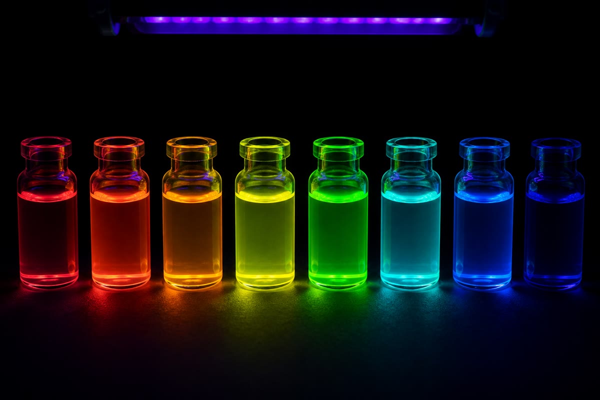
The 2023 Nobel Prize in Chemistry went to the discovery and synthesis of quantum dots: crystallites so small that the particle-in-a-box energies of this chapter set their colour, now glowing in television screens and tagging molecules in living cells. This problem designs a dot display from the Schrödinger equation. Model: the optically active electron–hole pair, effective mass $\mu = 0.10\,m_{\text{e}}$ ( $m_{\text{e}}c^2 = 511\,\mathrm{keV}$ ), confined in a sphere of radius $R$ ; emitted photon energy

E(R) = E_{\text{g}} + \frac{\pi^2\hbar^2}{2\mu R^2} ,

with the bulk band gap $E_{\text{g}} = 1.74\,\mathrm{eV}$ (cadmium selenide). Use $\hbar c = 197.3\,\mathrm{eV}\,\mathrm{nm}$ , $hc = 1240\,\mathrm{eV}\,\mathrm{nm}$ .

Part I — The physics of the formula.

Where does the term $\pi^2\hbar^2/2\mu R^2$ come from? Derive it as the ground level of the infinite spherical well via the $s$ -wave substitution.
Why does confinement always raise the emitted energy, never lower it?
Evaluate the confinement energy for $R = 10$ , $4$ , $2$ and $1\,\mathrm{nm}$ , and identify the size at which it stops being a small correction to $E_{\text{g}}$ .
The model ignores the electron–hole attraction. In which direction would including it shift the emission, and why is the neglect better for small dots (compare the $1/R^2$ and $1/R$ scalings)?
Bulk cadmium selenide emits at what wavelength? In which part of the spectrum does it lie?
Why does a glass of dot solution glow in one pure colour although it contains $10^{15}$ dots? What property of the synthesis is being certified?

Part II — Designing the palette. A display needs red $630\,\mathrm{nm}$ , green $530\,\mathrm{nm}$ , blue $460\,\mathrm{nm}$ .

Convert each wavelength to a photon energy.
For each colour, compute the required confinement energy and the dot radius.
Tabulate: how many atoms across is each dot, roughly (lattice spacing $\approx 0.6\,\mathrm{nm}$ )?
Blue proves hardest for cadmium selenide dots: from your radii, explain why (what happens to the tolerance as $R$ shrinks?).
Show that the sensitivity of the emitted energy to size is

$\frac{\dd E}{\dd R} = -\frac{\pi^2\hbar^2}{\mu R^3} ,$

and evaluate it, in $\mathrm{meV}$ per nanometre, at the green dot’s radius.
A batch varies by $\pm5\%$ in radius: compute the wavelength spread of the green emission, and compare with the $\sim25\,\mathrm{nm}$ linewidth a good display tolerates.
Why did quantum-dot displays have to wait for chemistry capable of atomic-scale size control — and why is that a Nobel-grade achievement?

Part III — Brighter, purer, stranger.

Modern sets use dots as colour converters: a blue LED illuminates red and green dots. Why must the pump photon’s energy exceed the dot’s emission energy, and where does the difference go?
Compute the fraction of a $460\,\mathrm{nm}$ pump photon’s energy lost as heat when a $630\,\mathrm{nm}$ red photon is emitted.
A dot can also absorb at many wavelengths but emit at one: explain, from the level structure, why absorption is broadband and emission narrow.
Biologists tag proteins with dots of several sizes excited by one ultraviolet lamp: what property of the dots makes one lamp suffice where organic dyes need one laser per colour?
Estimate the number of atoms in the red dot ( $4/3\pi R^3$ , atomic volume $\sim(0.3\,\mathrm{nm})^3$ ): is “artificial atom” a fair name for an object this size with discrete levels?
In one sentence: what plays the role of the “nucleus” in this artificial atom — what holds the electron?

Part IV — Confinement across physics.

The same estimate $E_1 \sim \pi^2\hbar^2/2MR^2$ applied to a nucleon in $R = 3\,\mathrm{fm}$ gives what energy scale? (It is why nuclear physics speaks MeV.)
Applied to an electron confined to nuclear size, it gives what scandalous energy — and what does that argue about electrons “inside” the nucleus (an argument that once killed a theory of beta decay)?
Applied to you ( $70\,\mathrm{kg}$ ) in a $2\,\mathrm{m}$ room: compute the confinement energy and conclude.
Invert the formula: at what confinement size does an electron’s confinement energy reach its rest energy $m_{\text{e}}c^2$ — and what new physics (creation of particle pairs, Chapter 5) warns that the single-particle Schrödinger equation is then out of its depth?
State the general scaling law: confinement energy versus mass and versus size.
Summarise the named result: one formula, $E_{\text{g}} + \pi^2\hbar^2/2\mu R^2$ , turns radii of $4.0$ , $2.5$ and $2.0\,\mathrm{nm}$ into red, green and blue — colour engineered by counting nanometres, on sale in any electronics shop.

Solution

Solution of Problem 7.1.

1. $s$ -wave: $u = rR$ obeys the free 1D equation inside the sphere with $u(0) = u(R) = 0$ : $u \propto \sin(\pi r/R)$ , energy $\pi^2\hbar^2/2\mu R^2$ . 2. The ground energy of a box is positive and grows as the box shrinks — localisation always costs kinetic energy (uncertainty principle); it can only add to the gap. 3. With $\pi^2(\hbar c)^2/2\mu c^2 = 3.76\,\mathrm{eV}\,\mathrm{nm}^{2}$ : $0.04$ , $0.24$ , $0.94$ , $3.8\,\mathrm{eV}$ — at $R \approx 2\,\mathrm{nm}$ the correction rivals the gap itself. 4. Attraction lowers the pair’s energy: emission shifts red. It scales as $1/R$ against the confinement’s $1/R^2$ : for small dots the box term wins and the neglect improves. 5. $1240/1.74 = 713\,\mathrm{nm}$ : at the red edge of vision. 6. One colour from $10^{15}$ emitters certifies that the synthesis made them all the same size — monodispersity, the chemical feat behind the physics. 7. $1.97$ , $2.34$ , $2.70\,\mathrm{eV}$ . 8. Confinement $0.23$ , $0.60$ , $0.96\,\mathrm{eV}$ : $R = \sqrt{3.76/\Delta E}$ gives $4.0$ , $2.5$ , $2.0\,\mathrm{nm}$ . 9. Diameters $8.1$ , $5.0$ , $4.0\,\mathrm{nm}$ : roughly $13$ , $8$ and $7$ lattice spacings across. 10. The blue dot is smallest, where $E$ depends most steeply on $R$ : a one-lattice-plane error shifts the colour most — small dots are the least forgiving. 11. Differentiate: $\dd E/\dd R = -2\Delta E_{\text{conf}}/R = -\pi^2\hbar^2/\mu R^3$ ; at $R = 2.5\,\mathrm{nm}$ : $2 \times 0.60/2.5 = 0.48\,\mathrm{eV}/\mathrm{nm} = 480\,\mathrm{meV}/\mathrm{nm}$ . 12. $\pm 5\% = \pm0.125\,\mathrm{nm}$ : $\Delta E = \pm 60\,\mathrm{meV}$ , i.e. $\Delta\lambda = \lambda^2\Delta E/hc \approx \pm14\,\mathrm{nm}$ — a $\sim28\,\mathrm{nm}$ spread, right at the display’s tolerance: five per cent is the boundary of acceptable chemistry. 13. Because colour purity demands size control at the single-lattice-plane level across $10^{15}$ particles — the controlled growth achieved by Ekimov, Brus and Bawendi, and cited by the 2023 Nobel committee. 14. A dot can only emit at its own (lowest) gap; absorbing requires at least that energy, so the pump must be bluer. The excess relaxes as lattice vibrations: heat. 15. $1 - 460/630 = 27\%$ of each pump photon’s energy heats the screen. 16. Above the emitting level the dot’s spectrum is dense (many box states): absorption succeeds over a broad band; the excitation then tumbles to the lowest excited state, and emission happens from that single level: narrow. 17. All dots absorb the same ultraviolet happily (broadband), while each size emits its own colour: one lamp, many labels — the inverse of dye chemistry. 18. $\tfrac43\pi(4.0)^3/(0.3)^3 \approx 10^{4}$ atoms: ten thousand atoms sharing one set of discrete, hydrogen-like levels — “artificial atom” is earned. 19. The crystal boundary: the confining wall of the semiconductor grain replaces the nucleus’s attraction as the agent that holds and quantises the electron. 20. $\pi^2(\hbar c)^2/2Mc^2R^2 = 384210/(2 \times 939 \times 9) \approx 23\,\mathrm{MeV}$ : nuclear physics speaks MeV because femtometre boxes do. 21. For an electron the box estimate turns relativistic; honestly, $E \sim \pi\hbar c/R \approx 200\,\mathrm{MeV}$ — yet beta electrons emerge with a few MeV: electrons cannot be constituents of nuclei, the argument that buried the old nuclear-electron model and prepared the neutrino’s invention. 22. $\pi^2\hbar^2/2ML^2 \approx 2 \times 10^{-70}\,\mathrm{J}$ : thirty-nine orders below thermal noise — people are not quantum confined. 23. $\pi^2\hbar^2/2m_{\text{e}}R^2 = m_{\text{e}}c^2$ at $R = \pi\hbar/\sqrt2\,m_{\text{e}}c \approx 0.9\,\mathrm{pm}$ , the Compton scale: there the confinement energy suffices to create electron–positron pairs and the one-particle equation abdicates to quantum field theory. 24. $E_{\text{conf}} \propto 1/MR^2$ : lighter particles and smaller boxes are more quantum, in one formula. 25. $E_{\text{g}} + \pi^2\hbar^2/2\mu R^2$ maps $4.0 \to$ red, $2.5 \to$ green, $2.0\,\mathrm{nm} \to$ blue: the particle-in-a-box, tuned by chemists to the nanometre, lights the shop window — confinement quantisation as consumer electronics.

Terms defined in this chapter

Wave function and probability in three dimensions

See all 431 terms in the glossary