University Physics — Year 3 · Bachelor Year 3

11The Hydrogen Atom

Nine-tenths of the atoms in the universe are hydrogen: one proton holding one electron, the only atom physics can solve exactly — and the key that opened every other. The old quantum theory of Chapter 2 guessed its energies; the machinery is now in place to derive them: the Coulomb potential enters the radial equation of the last chapter, and out come the levels $-E_{\text{I}}/n^2$ , the Bohr radius, the shells and subshells of chemistry’s periodic table, and the spectral series astronomers read in every nebula. The same solution, rescaled, describes ionised helium, muonic atoms, positronium, and the electron–hole “atoms” inside semiconductors; stretched to $n \approx 100$ it describes Rydberg atoms half a micrometre across, whose radio whispers map the Galaxy’s ionised clouds and whose interactions now drive quantum computers.

11.1 The Coulomb problem solved

Theorem 11.1 (Levels of hydrogen)

For $V(r) = -e^2/4\pi\varepsilon_0 r$ (write $k = e^2/4\pi \varepsilon_0$ ), the bound states are labelled $(n, l, m)$ with

E_n = -\frac{E_{\text{I}}}{n^2} , \qquad E_{\text{I}} = \frac{m_{\text{e}}k^2}{2\hbar^2} = 13.6\,\mathrm{eV} , \qquad n = 1, 2, 3, \dots

and, for each $n$ , the orbital numbers $l = 0, 1, \dots, n-1$ and $m = -l, \dots, l$ . The natural length is the Bohr radius $a_0 = \hbar^2/m_{\text{e}}k = 52.9\,\mathrm{pm}$ ; the ground state is

\psi_{100} = \frac{1}{\sqrt{\pi a_0^3}}\;\eu^{-r/a_0} .

The energy depends on $n$ alone: counting the $m$ ’s and $l$ ’s, level $n$ is $n^2$ -fold degenerate (doubled by spin, Chapter 12) — far beyond the $(2l+1)$ -fold degeneracy that isotropy explains.

Partial proof. For the ground state, try $u = Cr\,\eu^{-r/a}$ in the radial equation with $l = 0$ : $u'' = (1/a^2 - 2/ar)u$ , so $-\tfrac{\hbar^2}{2m_{\text{e}}}u'' - \tfrac kr u = Eu$ requires $\hbar^2/m_{\text{e}}a = k$ (matching the $1/r$ terms) — which is $a = a_0$ — and $E = -\hbar^2/2m_{\text{e}}a_0^2 = -E_{\text{I}}$ . The general solution (Laguerre polynomials, $n - l - 1$ radial nodes) is admitted; each step of the construction is elementary but long. The “accidental” $l$ -degeneracy mirrors a classical secret of the pure $1/r$ force — Kepler ellipses do not precess, and an extra conserved vector (Laplace–Runge–Lenz) points along the fixed major axis; its quantum version is what ties different $l$ to one energy (Exercise 11.12). ∎

The hydrogen levels -E_ I/n2, spread by l: all subshells of one n coincide (the Coulomb “accident”). Downward jumps ending on n = 1 form the ultraviolet Lyman series; those ending on n = 2, the visible Balmer series that colours nebulae red. — The hydrogen levels $-E_{\text{I}}/n^2$ , spread by $l$ : all subshells of one $n$ coincide (the Coulomb “accident”). Downward jumps ending on $n = 1$ form the ultraviolet Lyman series; those ending on $n = 2$ , the visible Balmer series that colours nebulae red.

11.2 Where the electron is

Proposition 11.2 (Radial distributions)

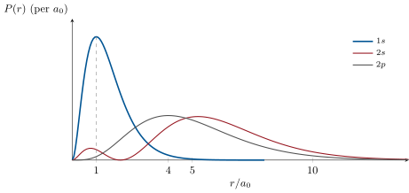
The probability of finding the electron between $r$ and $r + \dd r$ is $P(r)\,\dd r$ with $P(r) = |u(r)|^2$ , the square of the normalised radial function of Theorem 10.6. For the lowest states: $P_{1s} \propto r^2\eu^{-2r/a_0}$ , peaking at exactly $r = a_0$ with $\langle r\rangle = \tfrac32 a_0$ ; $P_{2s}$ shows two humps separated by a spherical node; $P_{2p} \propto r^4\eu^{-r/a_0}$ , peaking at $4a_0$ . Generally $\langle r\rangle \approx n^2a_0$ : atoms grow quadratically with excitation, while their binding shrinks as $1/n^2$ — the leverage behind the Rydberg giants of Problem 11.1.

Proof. Admitted at this level. ∎

Radial probability densities. The

1s

peak sits at exactly

a_0

; the

2s

state carries a spherical node and a lobe close to the nucleus — the “penetration” that will order the periodic table — while

2p

, walled off by the centrifugal barrier, keeps away.

Example 11.3 (Reading the sizes)

Ground state: $0.1\,\mathrm{nm}$ across, $13.6\,\mathrm{eV}$ deep — the scales of all chemistry. At $n = 10$ : radius $\sim5\,\mathrm{nm}$ , binding $0.136\,\mathrm{eV}$ — loosely held. At $n = 100$ : a micrometre-scale atom bound by $1.4\,\mathrm{meV}$ , wrecked by the feeblest field — yet interstellar space is empty enough for such atoms to live and broadcast (Problem 11.1).

11.3 The spectrum

Proposition 11.4 (Series and selection rules)

A jump $n' \to n$ emits the wavelength

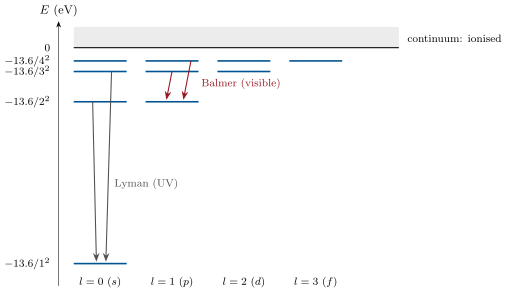
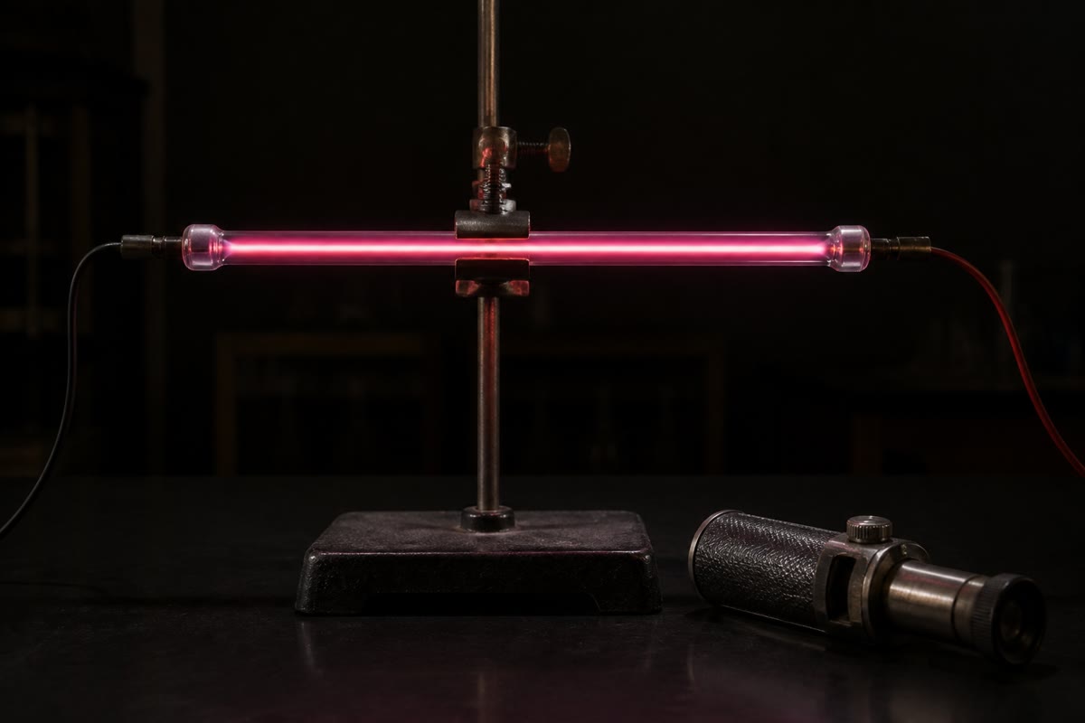
\frac{1}{\lambda} = R_{\text{H}}\Big(\frac{1}{n^2} - \frac{1}{n'^2}\Big) , \qquad R_{\text{H}} = \frac{E_{\text{I}}}{hc} = 1.097 \times 10^{7}\,\mathrm{m}^{-1} ,

subject to the dipole selection rule $\Delta l = \pm1$ (the photon carries $\hbar$ ). The Lyman series ( $\to n = 1$ ) lies in the far ultraviolet from $121.6\,\mathrm{nm}$ ; the Balmer series ( $\to n = 2$ ) begins at the red $H\alpha$ line, $656.3\,\mathrm{nm}$ — the colour of emission nebulae and solar prominences; the Paschen and later series recede into the infrared, and between $n = 110$ and $109$ the same formula lands at $5.0\,\mathrm{GHz}$ : hydrogen speaks from the ultraviolet to the radio dial.

Proof. Energy conservation with Theorem 11.1; $R_{\text{H}}$ as in Problem 2.1, now derived rather than postulated. ∎

Example 11.5 (Hydrogen-like atoms: one solution, many atoms)

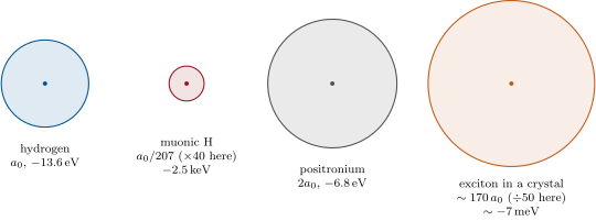
Replace the proton’s charge by $Ze$ and the electron by any orbiting mass $\mu$ : every formula rescales as

a \to a_0\,\frac{m_{\text{e}}}{\mu}\,\frac1Z , \qquad E_{\text{I}} \to E_{\text{I}}\,\frac{\mu}{m_{\text{e}}}\,Z^2 .

He $^+$ ( $Z = 2$ ): $54.4\,\mathrm{eV}$ . Inner electrons of heavy atoms ( $Z \sim 30$ ): K-shell energies in the keV — the characteristic X-rays by which Moseley ordered the elements (Exercise 11.5). Muonic hydrogen ( $\mu = 207 m_{\text{e}}$ ): a femtometre-scale atom probing the proton itself. Positronium ( $e^+e^-$ , $\mu = m_{\text{e}}/2$ ): half the binding, twice the size, and a short life ending in annihilation photons. And in a semiconductor, an electron and a hole orbit each other with small effective masses in a screening dielectric: an exciton, the same atom grown to ten nanometres and millielectronvolts (Exercise 11.7) — hydrogen is less an atom than a template.

One solution, four “atoms”: rescaling mass, charge and dielectric surroundings turns hydrogen into probes of the proton, tests of pure quantum electrodynamics, and the light-emitting quasi-atoms of semiconductors.

Method 11.6 (Working with hydrogenic systems)

(1) Scale first: $a \propto 1/\mu Z$ , $E \propto \mu Z^2$ turn any hydrogen answer into any hydrogen-like answer. (2) Sizes: $\langle r\rangle \sim n^2a$ ; spacings near level $n$ : $\dd E/\dd n = 2E_{\text{I}}/n^3$ . (3) Spectra: Rydberg formula plus $\Delta l = \pm1$ . (4) Penetration: $s$ states feel the nucleus, high- $l$ states orbit outside — the lever of multi-electron chemistry. (5) Sanity anchors: $13.6\,\mathrm{eV}$ , $52.9\,\mathrm{pm}$ , $121.6\,\mathrm{nm}$ , $656.3\,\mathrm{nm}$ — four numbers worth memorising for life.

A hydrogen discharge tube and a pocket spectroscope: the pink glow, split, becomes the Balmer lines — the integer fingerprint this chapter derives from the Coulomb potential.

11.4 Exercises

Exercise 11.1 ★

(a) Verify by substitution that $u = Cr\eu^{-r/a_0}$ solves the $l = 0$ radial equation with $E = -E_{\text{I}}$ , provided $a_0 = \hbar^2/m_{\text{e}}k$ . (b) Normalise it ( $\int_0^\infty x^2\eu^{-x}\dd x = 2$ ). (c) Check the dimensions of $a_0$ and $E_{\text{I}}$ . (d) Why is there no state below $-E_{\text{I}}$ (argue with Exercise 7.12)?

Solution

Solution of Exercise 11.1.

(a) $u'' = (1/a^2 - 2/ar)u$ ; the $1/r$ terms match when $\hbar^2/m_{\text{e}}a = k$ , i.e. $a = a_0$ , and the constant terms give $E = -\hbar^2/2m_{\text{e}}a_0^2 = -E_{\text{I}}$ . (b) $C = 2/a_0^{3/2}$ . (c) $[\hbar^2/mk] = \mathrm{m}$ ; $[mk^2/\hbar^2] = \mathrm{J}$ . (d) The variational argument of Exercise 7.12 shows $-E_{\text{I}}$ is the least energy any normalised state can achieve: the uncertainty principle floors the atom.

Exercise 11.2 ★

Compute (a) the wavelengths of Lyman $\alpha$ and of the Lyman limit; (b) the first three Balmer lines and the Balmer limit — which are visible, and what colours? (c) the Paschen series’ range; (d) the frequency of the $n = 110 \to 109$ transition.

Solution

Solution of Exercise 11.2.

(a) $121.6\,\mathrm{nm}$ ; limit $91.2\,\mathrm{nm}$ . (b) $656.3$ (red), $486.1$ (blue-green), $434.0\,\mathrm{nm}$ (violet); limit $364.6\,\mathrm{nm}$ — the first three are visible. (c) From $1875\,\mathrm{nm}$ down to $820\,\mathrm{nm}$ : near infrared. (d) $R_{\text{H}}c\,(1/109^2 - 1/110^2) = 5.01\,\mathrm{GHz}$ .

Exercise 11.3 ★

For the ground state: (a) locate the maximum of $P_{1s}(r)$ ; (b) compute $\langle r\rangle$ ; (c) compute the probability of finding the electron beyond $2a_0$ ( $\int_x^\infty t^2\eu^{-t}\dd t = (x^2 + 2x + 2)\eu^{-x}$ ); (d) why do “orbit” pictures at radius exactly $a_0$ mislead?

Solution

Solution of Exercise 11.3.

(a) $\dd(r^2\eu^{-2r/a_0})/\dd r = 0$ at $r = a_0$ . (b) $\langle r\rangle = (4/a_0^3)\int_0^\infty r^3\eu^{-2r/a_0}\dd r = (4/a_0^3)\times 3!\,(a_0/2)^4 = \tfrac32 a_0$ . (c) With $x = 4$ : $\tfrac12(16 + 8 + 2)\eu^{-4} = 0.24$ : a quarter of the time the electron is beyond $2a_0$ . (d) The electron has no radius: $P(r)$ is a distribution with a mode, a mean and long tails — the atom is fuzzy at the factor-two level.

Exercise 11.4 ★

(a) List the $(l, m)$ pairs of $n = 3$ and verify the count $n^2 = 9$ . (b) With spin, how many states in shells $n = 1, 2, 3$ ? (c) Match to the lengths $2, 8, 18$ of the periodic table’s rows. (d) Which degeneracy (in $m$ , or in $l$ ) survives in the outer electron of sodium, and why does the other break?

Solution

Solution of Exercise 11.4.

(a) $l = 0$ : one; $l = 1$ : three; $l = 2$ : five — nine. (b) $2$ , $8$ , $18$ . (c) Exactly the lengths of the first three rows: the periodic table is the filling record of these shells. (d) The $m$ -degeneracy survives (space is still isotropic); the $l$ -degeneracy breaks because the screened potential seen by the valence electron is no longer pure $1/r$ — Exercise 11.8.

Exercise 11.5 ★★

Moseley’s ladder. An inner (K-shell) electron of an element $Z$ moves in a nearly bare nuclear field screened by the one other K electron: effective charge $\approx Z - 1$ . (a) Show the $2p \to 1s$ X-ray energy is approximately $\tfrac34(Z-1)^2E_{\text{I}}$ . (b) Evaluate for copper ( $Z = 29$ ) and compare with the measured K $\alpha$ at $8.05\,\mathrm{keV}$ . (c) Moseley (1913) plotted $\sqrt{\nu}$ against $Z$ and got straight lines: what did this prove about the meaning of atomic number? (d) Predict the K $\alpha$ energy of the then-missing element $Z = 43$ .

Solution

Solution of Exercise 11.5.

(a) Hydrogen-like with $Z - 1$ : $h\nu = (Z-1)^2E_{\text{I}}(1 - \tfrac14)$ . (b) $784 \times 10.2\,\mathrm{eV} = 8.0\,\mathrm{keV}$ — matching the measured K $\alpha$ of copper. (c) That the integer ordering the elements is the nuclear charge, not the atomic weight: gaps in Moseley’s lines located undiscovered elements. (d) $42^2 \times 10.2 = 18.0\,\mathrm{keV}$ — technetium, found decades later, obliged.

Exercise 11.6 ★★

Positronium. (a) Justify $\mu = m_{\text{e}}/2$ and give its binding energy and Bohr radius. (b) Its Lyman $\alpha$ wavelength. (c) Para-positronium annihilates into two photons: their energies and relative directions (from Chapter 5). (d) Where does medicine detect exactly this signature daily?

Solution

Solution of Exercise 11.6.

(a) Two equal masses: $\mu = m_{\text{e}}/2$ : binding $6.8\,\mathrm{eV}$ , radius $2a_0 = 0.106\,\mathrm{nm}$ . (b) $\tfrac34 \times 6.8 = 5.1\,\mathrm{eV}$ : $243\,\mathrm{nm}$ . (c) Two photons of $511\,\mathrm{keV}$ , back to back (momentum conservation at rest). (d) Positron-emission tomography: the pair of collinear $511\,\mathrm{keV}$ photons is the signal every PET ring triangulates.

Exercise 11.7 ★★

Excitons. In gallium arsenide, $\varepsilon_{\text{r}} = 12.9$ and the reduced effective mass is $\mu = 0.058\,m_{\text{e}}$ . (a) Show $a_{\text{ex}} = a_0\,\varepsilon_{\text{r}}\,m_{\text{e}}/\mu$ and evaluate. (b) The exciton binding energy. (c) Compare $a_{\text{ex}}$ with the quantum-dot radii of Problem 7.1 and justify, at last, neglecting the Coulomb term in small dots. (d) Why do excitonic lines appear only in pure, cold semiconductors ( $k_{\text{B}}T$ against your answer to (b))?

Solution

Solution of Exercise 11.7.

(a) $a_{\text{ex}} = 0.0529 \times 12.9/0.058 = 11.8\,\mathrm{nm}$ . (b) $E = 13.6 \times 0.058/12.9^2 = 4.7\,\mathrm{meV}$ . (c) The natural pair size exceeds the dot: the wall, not the attraction, shapes the state — the $1/R^2$ beats the $1/R$ , as promised. (d) $k_{\text{B}}T$ at room temperature is five times the binding: the pairs ionise; excitonic physics lives below $\sim50\,\mathrm{K}$ in clean crystals.

Exercise 11.8 ★★

Penetration and the alkali metals. Sodium is a hydrogen-like valence electron outside a closed core of charge $+e$ effective. (a) Which of $3s$ , $3p$ , $3d$ feels the incompletely screened nucleus most, and why (recall the radial figure)? (b) The measured levels are $E_{3s} = -5.14\,\mathrm{eV}$ , $E_{3p} = -3.04\,\mathrm{eV}, E_{3d} = -1.52\,\mathrm{eV}$ : check that $3d$ is nearly hydrogenic ( $n = 3$ ) while $3s$ is far deeper, and explain. (c) Compute the wavelength of $3p \to 3s$ : what famous colour is that? (d) Write the alkali levels as $-E_{\text{I}}/(n - \delta_l)^2$ and extract the “quantum defects” $\delta_s$ and $\delta_p$ for sodium.

Solution

Solution of Exercise 11.8.

(a) $3s$ : its innermost lobe dives inside the core where the nuclear $+11$ is barely screened. (b) $-13.6/9 = -1.51\,\mathrm{eV}$ matches $3d$ almost exactly: $3d$ orbits outside the core and sees a net $+1$ ; $3s$ (and partly $3p$ ) taste the deep potential and sink. (c) $\Delta E = 2.10\,\mathrm{eV}$ : $\lambda = 590\,\mathrm{nm}$ — the sodium yellow of street lamps. (d) $n_{\text{eff}} = \sqrt{13.6/|E|}$ : $1.63$ and $2.11$ , so $\delta_s = 1.37$ , $\delta_p = 0.89$ .

Exercise 11.9 ★★

A proton in a nebula captures an electron into $n = 100$ . (a) How much energy is released in the capture photon if the electron arrived nearly free? (b) The atom cascades down, preferentially by $\Delta n = 1$ steps at high $n$ : in which band do those photons fall? (c) The cascade’s last step is Lyman $\alpha$ ; the visible light of nebulae is dominated by H $\alpha$ : trace which cascade step that is. (d) Explain why emission nebulae glow red although hydrogen’s strongest line (Lyman $\alpha$ ) is ultraviolet.

Solution

Solution of Exercise 11.9.

(a) About the binding of $n = 100$ , $\sim1.4\,\mathrm{meV}$ , plus the electron’s small thermal energy: a far-infrared/radio photon. (b) The $\Delta n = 1$ steps near $n \approx 100$ fall in the GHz radio band — the recombination lines. (c) H $\alpha$ is the step $3 \to 2$ , near the cascade’s end. (d) Lyman $\alpha$ , though strongest, is ultraviolet and, in a nebula full of ground-state hydrogen, is resonantly scattered and trapped; H $\alpha$ escapes freely and paints the nebula red.

Exercise 11.10 ★★★

Averages and the virial. For the ground state, compute (a) $\langle 1/r\rangle$ and check $\langle E_p\rangle = -2E_{\text{I}} = 2E_1$ ; (b) $\langle E_k\rangle = +E_{\text{I}}$ , verifying the virial ratio of Exercise 2.4; (c) the electron’s r.m.s. speed and $v/c$ ; (d) the order of magnitude of the magnetic field that the proton experiences from the electron’s motion (a current loop $ev/2\pi a_0$ seen at distance $a_0$ ) — a number hyperfine structure will need.

Solution

Solution of Exercise 11.10.

(a) $\langle 1/r\rangle = 1/a_0$ : $\langle E_p\rangle = -k/a_0 = -27.2\,\mathrm{eV} = 2E_1$ . (b) $\langle E_k\rangle = E_1 - \langle E_p\rangle = +13.6\,\mathrm{eV}$ : the virial ratio $-\tfrac12$ of every $1/r$ orbit. (c) $v = \sqrt{2E_k/m_{\text{e}}} = \alpha c = 2.2 \times 10^{6}\,\mathrm{m}/\mathrm{s}$ . (d) $I = ev/2\pi a_0 \approx 1\,\mathrm{mA}$ circulating at $53\,\mathrm{pm}$ : $B \sim \mu_0I/2a_0 \approx 12\,\mathrm{T}$ — the enormous internal field hyperfine structure will feed on.

Exercise 11.11 ★★★

How fine is fine structure. (a) Show the ground-state speed scale is $\langle v^2\rangle^{1/2}/c = \alpha \approx 1/137$ , and for hydrogen-like $Z$ : $Z\alpha/n$ . (b) Relativistic corrections enter at relative order $(v/c)^2$ : estimate the fine-structure scale $\alpha^2E_{\text{I}}$ in meV, and the splitting’s order for $n = 2$ in GHz. (c) For hydrogen-like uranium ( $Z = 92$ ): $v/c$ at $n = 1$ — is the non-relativistic treatment tenable? (d) What does the formal divergence at $Z\alpha \to 1$ ( $Z \approx 137$ ) announce physically?

Solution

Solution of Exercise 11.11.

(a) From Exercise 11.10(c), $v/c = \alpha$ ; scaling: $Z\alpha/n$ . (b) $\alpha^2E_{\text{I}} = 0.72\,\mathrm{meV}$ ; at $n = 2$ the splittings come out tens of $\text{µ}\mathrm{eV}$ — some $10\,\mathrm{GHz}$ , radio-measurable (and measured). (c) $Z\alpha = 0.67$ : two-thirds of light speed — the Schrödinger treatment fails; Dirac’s equation takes over. (d) At $Z\alpha \to 1$ the ground state’s energy formally dives past $-2m_{\text{e}}c^2$ : the vacuum itself would spark electron–positron pairs — supercritical fields, sought in heavy-ion collisions.

Exercise 11.12 ★★★

The unreasonable degeneracy. (a) In classical mechanics, show that for $V = -k/r$ the orbit closes (no precession) by citing the conserved Laplace–Runge–Lenz vector $\vect A = \vect p\wedge\vect L - mk\,\vect e_r$ — verify $\dd\vect A/\dd t = 0$ using Newton’s law. (b) Argue: a conserved vector fixing the ellipse’s axis is an extra symmetry beyond rotations — and extra symmetry means extra degeneracy (recall Exercise 8.9). (c) Add a small $1/r^2$ correction to the potential and show the ellipse precesses: the axis turns, $\vect A$ is no longer conserved. (d) Connect: in multi-electron atoms the effective potential is not pure $1/r$ , and the $l$ -degeneracy breaks (sodium!); in hydrogen itself, relativity supplies the small correction — which observed feature of Exercise 11.11 is that?

Solution

Solution of Exercise 11.12.

(a) Differentiate: $\dot{\vect p}\wedge\vect L = -(mk/r^3)\vect r\wedge(\vect r\wedge\dot{\vect r}\,m)$ ; expanding the double cross product gives exactly $mk\,\dd\vect e_r/\dd t$ : $\dot{\vect A} = \vect 0$ . (b) A conserved axis is a symmetry beyond isotropy; degeneracy is incomplete labelling, and the extra label ( $\vect A$ ’s quantum cousin) connects the $l$ ’s within one $n$ . (c) With $V = -k/r + \epsilon/r^2$ the effective angular momentum shifts, the angular period no longer matches the radial one, and the ellipse’s axis turns at a rate $\propto\epsilon$ . (d) Relativity’s corrections play the role of $\epsilon$ in hydrogen itself: the fine structure of Exercise 11.11 is precisely the $l$ -degeneracy breaking.

11.5 Problem: Giant atoms

Problem 11.1

Weekend problem — Rydberg atoms, from the Galaxy’s radio glow to quantum computers

Stretch hydrogen to $n \approx 100$ and it becomes a different kind of object: micrometres across, bound by millielectronvolts, absurdly sensitive — and absurdly useful. This problem scales the hydrogen solution up, first to the interstellar clouds that broadcast at centimetre wavelengths, then to the laboratory arrays where such giants entangle each other into processors. Data: $E_{\text{I}} = 13.6\,\mathrm{eV}$ , $a_0 = 52.9\,\mathrm{pm}$ , $R_{\text{H}}c = 3.29 \times 10^{15}\,\mathrm{Hz}$ , $k_{\text{B}}T$ at $300\,\mathrm{K}$ is $25.9\,\mathrm{meV}$ .

Part I — The scaling laws.

Give the four basic scalings with $n$ : size $\langle r\rangle$ , binding $|E_n|$ , spacing $E_{n+1} - E_n$ (for large $n$ ), and the classical orbital frequency of the corresponding Bohr orbit.
Show that for large $n$ the transition frequency $n+1 \to n$ approaches $2R_{\text{H}}c/n^3$ , and verify it equals the classical orbital frequency (the correspondence principle of Problem 2.1, completed).
Evaluate size and binding at $n = 50$ and $n = 100$ .
The electric dipole of a Rydberg atom scales as $n^2ea_0$ : evaluate at $n = 50$ in debye ( $1\,\text{D} = 3.34 \times 10^{-30}\,\mathrm{C}\,\mathrm{m}$ ) and compare with a water molecule’s $1.85\,\mathrm{D}$ .
Estimate the electric field that rips the $n = 50$ atom apart, as $F \sim |E_n|/(e\,\langle r\rangle)$ , in V/cm.
Why can such atoms not survive ordinary laboratory vacuum chemistry — yet survive fine in interstellar space (compare collision rates)?

Part II — The Galaxy’s recombination lines. In ionised nebulae, protons capture electrons into high $n$ ; the cascade radiates a comb of “radio recombination lines”.

Compute the frequency of the $n = 110 \to 109$ transition (called H109 $\alpha$ ).
In what band does it fall, and what kind of telescope receives it?
Compute the wavelength of H109 $\alpha$ and compare it with the size of the emitting atom: how many atoms fit in one wavelength?
These lines measure the nebula’s temperature by their Doppler width: at $T = 10^{4}\,\mathrm{K}$ , the hydrogen thermal speed is $\sim12.8\,\mathrm{km}/\mathrm{s}$ — compute the fractional linewidth $\Delta\nu/\nu$ and the width of H109 $\alpha$ in kHz.
Radio waves cross the dust that blackens the optical sky: what does that let recombination-line astronomers map that Balmer-line astronomers cannot?
Above roughly $n \sim 1000$ (atoms $0.05$ millimetres across!), the levels blur into a continuum even in space: name two effects that broaden or destroy such states.

Part III — Giants in the laboratory.

Lasers drive rubidium atoms to $n \approx 70$ in micrometre-spaced optical-tweezer arrays. Two such atoms a distance $R$ apart interact by their induced dipoles (recall Exercise 9.10): with dipole $\propto n^2$ , show the van der Waals strength scales as a colossal $n^{11}$ (use $C_6 \propto d^4/\Delta E$ with level spacing $\Delta E \propto n^{-3}$ ).
The “blockade”: within a radius $R_{\text{b}}$ , the interaction shifts the doubly excited state out of laser resonance, so two atoms cannot both be excited. Explain in one sentence why this realises a two-qubit gate.
Blockade radii reach several micrometres — thousands of times the atoms’ ground-state size: why is this long reach (compare chemistry’s nanometre range) exactly what a scalable processor wants?
A Rydberg state at $n = 70$ lives $\sim100\,\text{µ}\mathrm{s}$ while a gate takes $\sim0.5\,\text{µ}\mathrm{s}$ : roughly how many operations fit in one lifetime, and why does that ratio, not the lifetime alone, matter?
Room-temperature blackbody radiation, peaking near $100\,\mathrm{meV}$ but rich in a low-energy tail, drives transitions between neighbouring Rydberg levels spaced by only $\sim0.1\,\mathrm{meV}$ : why must precision experiments enclose the atoms in cold shields?
Estimate how many antenna-like dipole transitions ( $\propto n^2$ ) a $300\,\mathrm{K}$ photon bath drives per second compared with an $n = 1$ atom: which scaling makes Rydberg atoms exquisite sensors of microwave and terahertz fields?

Part IV — The big picture.

One formula, $E_n = -E_{\text{I}}\mu Z^2/m_{\text{e}}n^2$ , spans how many orders of magnitude of binding energy from hydrogen-like uranium ( $Z = 92$ , $n = 1$ ) down to an $n = 1000$ Rydberg state? Compute both ends.
Radiative lifetimes of low- $l$ states scale as $n^3$ : from the $2p$ lifetime of $1.6\,\mathrm{ns}$ , estimate the lifetime of a $100p$ state — and compare with the room-temperature blackbody problem of Part III.
At CERN, anti-atoms of antihydrogen are now spectroscopied on the $1s \to 2s$ interval to fifteen digits: what fundamental symmetry does agreement with ordinary hydrogen test, and why is hydrogen the right atom for the comparison?
At $n \sim 100$ the electron’s de Broglie wave wraps a nearly classical orbit; at $n = 1$ no orbit exists at all: in one sentence, where does the classical picture switch on?
Rydberg constants are measured to fifteen digits: why is hydrogen, of all systems, the natural precision anchor of atomic physics?
The 2012 Nobel Prize (Haroche) used Rydberg atoms as photon-counters that do not destroy the photon: which two properties from Part I and III make them ideal non-demolition probes of microwave fields?
Summarise the named result: the $n^2$ , $n^{-2}$ , $n^{-3}$ and $n^{11}$ scalings of one exactly solved atom stretch hydrogen from $52.9\,\mathrm{pm}$ to half a micrometre, tune its voice from $121.6\,\mathrm{nm}$ to $6\,\mathrm{cm}$ , and turn it into both the Galaxy’s radio beacon and the two-qubit gate of neutral-atom quantum computers.

Solution

Solution of Problem 11.1.

1. $\langle r\rangle \sim n^2a_0$ ; $|E_n| = E_{\text{I}}/n^2$ ; spacing $\approx 2E_{\text{I}}/n^3$ ; orbital frequency $\propto 1/n^3$ (Kepler on the Bohr orbit). 2. $E_{n+1} - E_n \to 2E_{\text{I}}/n^3$ , and $h$ times the classical frequency $v_n/2\pi r_n$ equals the same expression (the computation of Problem 2.1, item 20). 3. $n = 50$ : $132\,\mathrm{nm}$ , $5.4\,\mathrm{meV}$ ; $n = 100$ : $0.53\,\text{µ}\mathrm{m}$ , $1.4\,\mathrm{meV}$ . 4. $n^2ea_0 = 2.1 \times 10^{-26}\,\mathrm{C}\,\mathrm{m} \approx 6300\,\text{D}$ : three thousand water molecules’ worth of dipole on one atom. 5. $F \sim 5.4 \times 10^{-3}/1.32 \times 10^{-7} \approx 4 \times 10^{4}\,\mathrm{V}/\mathrm{m} = 400\,\mathrm{V}/\mathrm{cm}$ ; the exact classical-ionisation threshold is about eight times smaller ( $\sim50\,\mathrm{V}/\mathrm{cm}$ ): either way, a whisper of a field. 6. With geometric cross-sections $\sim\pi n^4a_0^2$ , even ultra-high laboratory vacuum collides such an atom in microseconds; interstellar densities ( $\sim10^{6}$ particles per $\mathrm{m}^{3}$ ) leave it days — space is the better vacuum chamber. 7. $\nu = R_{\text{H}}c\,(1/109^2 - 1/110^2) = 5.01\,\mathrm{GHz}$ . 8. Centimetre radio: a radio telescope — a big dish and a quiet receiver. 9. $\lambda = 6.0\,\mathrm{cm}$ ; the $n = 110$ atom is $\sim0.6\,\text{µ}\mathrm{m}$ : a hundred thousand atoms per wavelength — comfortably an “antenna” regime. 10. $\Delta\nu/\nu \sim v/c = 4.3 \times 10^{-5}$ : about $200\,\mathrm{kHz}$ on $5\,\mathrm{GHz}$ — and the measured width hands back the nebular temperature. 11. The ionised inner Galaxy: HII regions hidden behind dust that extinguishes every Balmer photon — radio recombination lines mapped the spiral structure optical astronomy could not see. 12. The micro electric fields of neighbouring ions (Stark broadening) smear the levels, and blackbody/cosmic radiation plus collisions ionise or $l$ -mix the fragile states. 13. $C_6 \sim d^4/\Delta E \propto (n^2)^4/n^{-3} = n^{11}$ : raise $n$ from $1$ to $70$ and the interaction grows by twenty orders of magnitude. 14. Within $R_{\text{b}}$ the pair state is shifted off resonance, so one atom’s excitation conditions its neighbour’s response: exactly the controlled logic a two-qubit gate needs. 15. Micrometre-range interactions let each atom sit in its own addressable tweezer, far apart by atomic standards yet strongly coupled — interaction range matched to optical resolution. 16. $\sim 200$ gates per lifetime: the ratio bounds the achievable fidelity, and it is the ratio, not the raw microseconds, that a processor lives on. 17. At $300\,\mathrm{K}$ the photon bath is dense at $\sim0.1\,\mathrm{meV}$ : it shuffles and ionises Rydberg levels within their radiative lifetimes; cold ( $4\,\mathrm{K}$ ) shields starve those transitions. 18. Transition rates scale as $d^2 \propto n^4$ : at $n = 50$ , six million times an ordinary atom’s coupling — which is why a vapour cell of Rydberg atoms is now a calibrated microwave and terahertz field sensor. 19. $92^2 \times 13.6\,\mathrm{eV} = 115\,\mathrm{keV}$ down to $13.6/10^6\,\mathrm{eV} = 13.6\,\text{µ}\mathrm{eV}$ : ten orders of magnitude from one formula. 20. Classicality dawns where the spacing becomes a vanishing fraction of the energy, $n \gg 1$ — the atom’s own correspondence limit. 21. It is the one atom computable from first principles to the experiment’s precision: any mismatch is discovery, so hydrogen anchors the fundamental constants. 22. $\tau \approx 1.6\,\mathrm{ns} \times 50^3 = 0.2\,\mathrm{ms}$ — generous, but blackbody redistribution (Part III) eats into it, another reason for the cold shields. 23. CPT symmetry — matter and antimatter atoms must match line by line; hydrogen is the anchor because only there does theory reach the fifteenth digit alongside experiment. 24. The $n^2$ dipole makes the atom feel a single microwave photon’s field, while its long lifetime and level structure let it acquire a measurable phase without absorbing the photon: quantum non-demolition sensing. 25. Scalings $n^2$ , $n^{-2}$ , $n^{-3}$ , $n^{11}$ stretch the one solved atom from $52.9\,\mathrm{pm}$ to half a micrometre and from $121.6\,\mathrm{nm}$ to $6\,\mathrm{cm}$ — the same Schrödinger solution broadcasting from the Galaxy’s HII regions and clocking two-qubit gates in tweezer arrays.