University Biology — Year 3 · Bachelor Year 3

27Conservation Biology

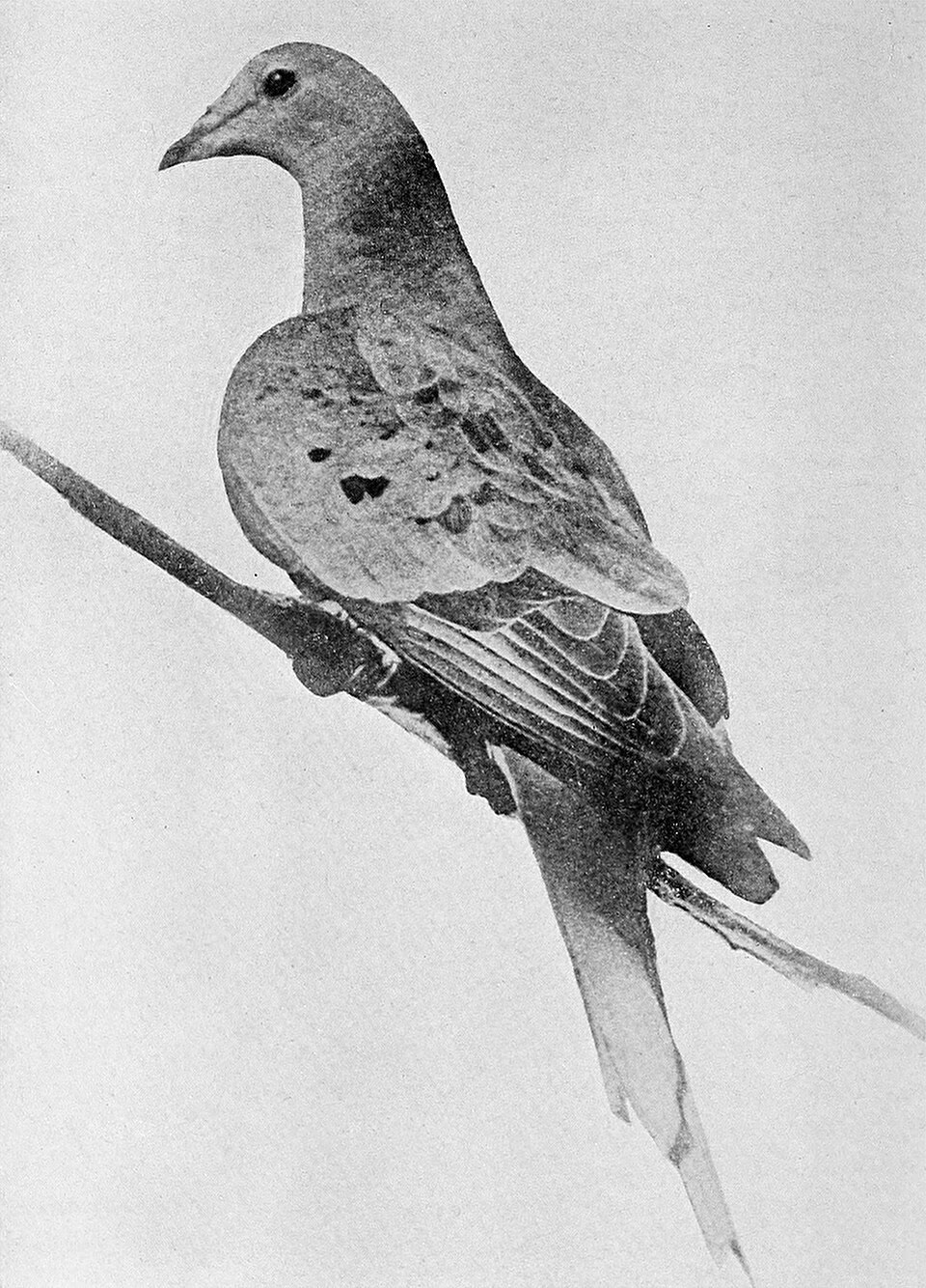
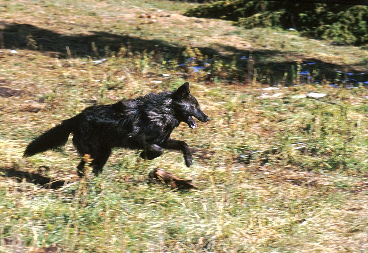
In 1813 Audubon watched a flock of passenger pigeons pass over Kentucky for three days, darkening the sky; there were perhaps five billion of them, a quarter of all the birds in North America. On 1 September 1914 the last one, a female named Martha, died in the Cincinnati Zoo. The species was not rare when its decline began; it was harvested by the trainload, and its forests were cut, and a bird that bred only in immense colonies could not breed once the colonies had thinned below some size no one measured. In 1995 the kakapo, a flightless nocturnal parrot of New Zealand, was down to fifty-one birds; every one has since been named, weighed, fitted with a transmitter and, at the right moment, offered a supplementary meal, and there are two hundred and fifty. In the same year thirty-one grey wolves were released into Yellowstone, seventy years after the last native pack had been shot; within two decades the elk had moved, the willows had come back along the rivers, and the beavers with them. Conservation biology is the application of this book’s population genetics, ecology and behaviour to a single practical question — how to keep species from disappearing — and its arithmetic is the arithmetic of small numbers.

27.1 Why small populations die

Definition 27.1 (The risks of smallness)

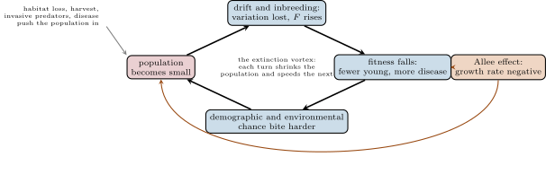
A large population declines when its death rate exceeds its birth rate; a small one can vanish without any change in either. Demographic stochasticity is the chance that, among a few individuals, more happen to die than are born, or all the survivors are male: it matters below a few dozen. Environmental stochasticity — a bad winter, a drought, a disease — strikes every individual at once, and a population of a few hundred that a large one would ride out can be wiped out; catastrophes are its tail. The Allee effect makes the per-capita growth rate fall at low density — mates cannot be found, colonial breeders cannot nest, herds cannot defend their young, the passenger pigeon’s flocks could not saturate the predators that took their squabs — so that below a threshold density the population declines toward zero on its own. And below a few hundred, the genetic processes of the next section reduce fitness generation by generation. These feed one another: a smaller population loses variation, becomes less fertile, grows smaller, is likelier to be hit by chance, and loses more — the extinction vortex (Gilpin and Soulé, 1986). A minimum viable population is the size above which the probability of extinction over a stated horizon (say $5\,\%$ in a century) is acceptable; it depends on the species’ biology and on how variable its environment is, and is usually in the thousands.

The extinction vortex. An external blow makes a population small; smallness then loses variation, lowers fitness, exposes the population to chance, and makes it smaller still. Conservation’s task is to break the loop before it closes.

Theorem 27.2 (Effective population size)

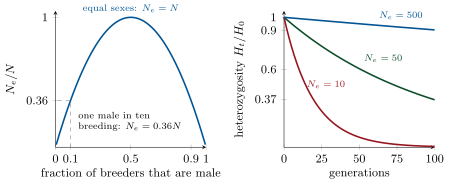
The rate at which a population loses variation and accumulates inbreeding is governed not by its census size $N$ but by its effective size $N_{e}$ : the size of an ideal population — constant, randomly mating, equal sex ratio, Poisson family sizes — that would lose heterozygosity at the same rate. Three departures from the ideal lower it. Unequal sex ratio, with $N_{m}$ breeding males and $N_{f}$ females:

N_{e} = \frac{4N_{m}N_{f}}{N_{m} + N_{f}} ;

one male and a hundred females give $N_{e} \approx 4$ . Fluctuating size over $t$ generations: $N_{e}$ is the harmonic mean of the generation sizes, $1/N_{e} = (1/t)\sum 1/N_{i}$ , dominated by the smallest — a population of a thousand that once passed through ten has $N_{e}$ near a hundred over that span. And variance in family size above Poisson lowers it further. In a population of effective size $N_{e}$ the inbreeding coefficient $F$ — the probability that the two alleles at a locus in an individual are copies of one ancestral allele — rises by $1/2N_{e}$ per generation,

F_{t} = 1 - \Bigl(1 - \frac{1}{2N_{e}}\Bigr)^{t} \approx \frac{t}{2N_{e}}, \qquad H_{t} = H_{0}\Bigl(1 - \frac{1}{2N_{e}}\Bigr)^{t} ,

and the heterozygosity $H$ decays at the same rate. Franklin’s rule of thumb, “50/500”: $N_{e} \ge 50$ keeps inbreeding below $1\,\%$ a generation, the rate animal breeders tolerate; $N_{e} \ge 500$ lets mutation replace the variation drift removes. Since $N_{e}$ is typically a tenth of the census size, the rule asks for populations of five hundred to five thousand.

Proof. Two gametes drawn at random from the population are copies of the same parental allele with probability $1/2N$ in the ideal population, which is $F$ ’s increment; heterozygosity is $1 - F$ scaled, so each generation multiplies it by $(1 - 1/2N_{e})$ , giving the exponential decay and, for $t \ll N_{e}$ , the linear rise of $F$ . Sex ratio: half the genes come from each sex, so the chance two gametes share a parental allele is $\tfrac{1}{4}\cdot\tfrac{1}{2N_{m}} + \tfrac{1}{4}\cdot\tfrac{1}{2N_{f}}$ (a quarter of pairs are both paternal, a quarter both maternal); setting this equal to $1/2N_{e}$ gives $1/N_{e} = 1/(4N_{m}) + 1/(4N_{f})$ , the formula. Fluctuation: heterozygosity after $t$ generations is $H_{0}\prod(1 - 1/2N_{i}) \approx H_{0}\exp(-\sum 1/2N_{i})$ , equal to $H_{0}\exp(-t/2N_{e})$ when $1/N_{e}$ is the average of the $1/N_{i}$ . Inbreeding lowers fitness because it exposes recessive deleterious alleles as homozygotes — inbreeding depression, a fall of several per cent in survival or fecundity per $10\,\%$ of $F$ in most outbreeding species. ∎

Left: how a skewed sex ratio shrinks the effective size — a harem species with a tenth of the males breeding has an N_e a third of its census. Right: heterozygosity decaying by (1 - 1/2N_e) per generation — a population of ten loses most of its variation in a century, one of five hundred almost none. — Left: how a skewed sex ratio shrinks the effective size — a harem species with a tenth of the males breeding has an $N_{e}$ a third of its census. Right: heterozygosity decaying by $(1 - 1/2N_{e})$ per generation — a population of ten loses most of its variation in a century, one of five hundred almost none.

Evidence. The Florida panther, down to some twenty-five animals in the 1990s, showed kinked tails, undescended testicles, heart defects and sperm of which $90\,\%$ were abnormal — inbreeding depression made visible; eight females introduced from Texas in 1995 (genetic rescue) tripled the population and the defects receded. The wolves of Isle Royale, founded by a pair in 1949 and isolated, declined to two grossly inbred individuals by 2018 with spinal deformities in most skeletons examined. The greater prairie chicken of Illinois fell from thousands to fifty, and its egg hatching rate from $93\,\%$ to $56\,\%$ , recovering after birds were brought from other states. Museum skins and ancient DNA let the loss of heterozygosity be measured directly against the pre-decline population in each case. ∎

Left: Martha, the last passenger pigeon, photographed in the Cincinnati Zoo in 1912; the species had numbered billions within living memory (photograph by Enno Meyer, public domain). Right: a cheetah — a species that passed through a bottleneck some ten thousand years ago and whose individuals are so alike that skin grafts between unrelated animals are not rejected.

27.2 Habitat: how much, and in what shape

Proposition 27.3 (Species and area)

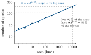
Across islands, and across habitat fragments that behave like islands, the number of species $S$ rises with area $A$ as a power law,

S = c\,A^{z}, \qquad z \approx 0.15\text{--}0.35,

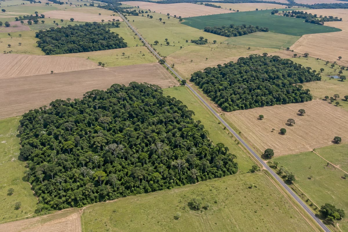
the species–area relationship (Arrhenius, 1921; MacArthur and Wilson’s island biogeography, 1967, explained it as a balance of immigration and extinction, extinction being faster on small islands). With $z = 0.25$ , losing $90\,\%$ of a habitat’s area eventually loses $1 - 0.1^{0.25} = 44\,\%$ of its species; losing half loses $16\,\%$ . The loss is not immediate — an extinction debt is paid over decades as populations too small for their fragments dwindle — and fragmentation of a fixed area into pieces adds losses of its own: each fragment holds a smaller population, edge effects (wind, heat, predators, weeds) penetrate hundreds of metres into forest, and species that need the interior lose more than the area accounts for. Whether a single large reserve or several small ones of the same total area saves more species (the SLOSS debate) depends on the species: the large one holds larger populations and interior habitat, the small ones spread the risk of a catastrophe and sample more habitat types. Corridors that connect fragments let individuals and genes move between them, turning isolated populations into a metapopulation whose parts can be recolonised after local extinction and rescued from inbreeding — which is why the land between reserves has become as much the concern as the reserves.

Proof. The power law is empirical, fitted on log–log axes to archipelagos, lakes, mountaintops and forest fragments the world over; the value of $z$ is lower for pieces of a mainland (immigration keeps species present) and higher for true islands. The fractional loss follows directly: $S'/S = (A'/A)^{z}$ . Island biogeography’s mechanism was tested by Simberloff and Wilson (1969), who fumigated small mangrove islets in Florida, killing every arthropod, and watched species numbers return to their previous values within a year — an equilibrium, with different species than before: the number is set by area and distance, the identities by chance. ∎

The species–area law on logarithmic axes. Its slope is the exponent z; from it the eventual loss of species from a shrunken habitat can be read — a tenth of the forest keeps about half the species, and not the tenth a linear guess would give. — The species–area law on logarithmic axes. Its slope is the exponent $z$ ; from it the eventual loss of species from a shrunken habitat can be read — a tenth of the forest keeps about half the species, and not the tenth a linear guess would give.

Forest fragments in farmland, seen from the air: each island holds a population smaller than the whole did, edged by a zone the interior species cannot use, and separated by fields the forest species cannot cross.

27.3 Predicting and preventing

Method 27.4 (Population viability analysis)

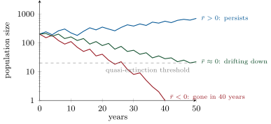
To estimate a population’s risk of extinction and what would reduce it: (1) build a model of its dynamics — a matrix of age- or stage-specific survival and fecundity, as in the Year 2 volume’s demography, estimated from marked individuals over several years; (2) add stochasticity — demographic, by drawing each individual’s fate at random, and environmental, by drawing each year’s rates from their observed variance, with occasional catastrophes; (3) add density dependence and the genetic decline of inbreeding where data allow; (4) simulate thousands of trajectories from the current size over the horizon of interest and record the fraction that fall below a quasi-extinction threshold (a size from which recovery is judged impossible); (5) vary the inputs — adult survival, juvenile survival, habitat area, a translocation of ten animals — and see which change most reduces the risk; that is where effort should go. The output is a probability with wide uncertainty, not a prediction; its value is comparative, and it has repeatedly shown that adult survival, not fecundity, is the lever in long-lived species, which is why fishing lines kill albatross populations that lay one egg every two years faster than any loss of nests could.

Proposition 27.5 (Time to extinction)

For a population that fluctuates because the environment does, with mean growth rate $\bar r$ near zero and variance $\sigma^{2}$ in the annual growth rate, the log of population size performs a random walk with drift, and the expected time to extinction from size $N$ grows only as the logarithm of $N$ when $\bar r < 0$ — doubling the population adds a fixed number of years — and as a power of $N$ when $\bar r > 0$ , with exponent $2\bar r/\sigma^{2} - 1$ ; under demographic stochasticity alone it grows exponentially with $N$ , so that a population safe from demographic chance at a hundred can still be lost to environmental variance at ten thousand. The practical consequence is that reducing the variance of a population’s growth — buffering it against bad years with more habitat, more sites, a wider diet — can do more for its persistence than raising its mean.

Proof. Admitted at this level. ∎

Three simulated trajectories from the same two hundred animals, differing only in mean growth rate; a viability analysis runs thousands of these and counts how many cross the threshold. The variance from year to year is what makes even the middle case a gamble.

Definition 27.6 (The tools)

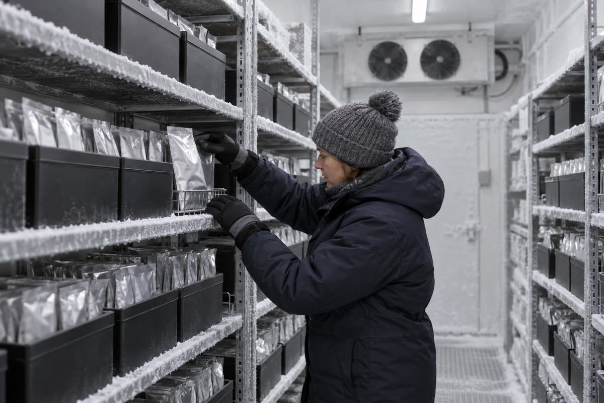
The IUCN Red List classifies species by quantitative criteria: a decline of $30\,\%$ , $50\,\%$ or $80\,\%$ over ten years or three generations, a range below $20\,000\,$ , $5000\,$ or $100\,\mathrm{km}^{2}$ , a population below $10\,000\,$ , $2500\,$ or $250\,$ mature individuals, or a modelled extinction probability, place a species as Vulnerable, Endangered or Critically Endangered; a quarter of mammals and an eighth of birds qualify. The causes are habitat loss first, then over-harvest, invasive species (predators and competitors carried to islands whose species had never met them: rats, cats and stoats have taken most of New Zealand’s birds, a single brown tree snake species most of Guam’s), pollution and climate change. The responses: protected areas covering a sixth of the land; the control or eradication of invaders (a hundred and fifty islands cleared of rats); ex situ conservation — seed banks holding a million accessions in a vault in the Arctic permafrost, frozen embryos, and captive breeding with pedigrees managed to minimise kinship, which brought the California condor back from twenty-two birds in 1987 and the black-footed ferret from eighteen; reintroduction, which succeeds about a third of the time and more often when the cause of the original loss has been removed; and rewilding, the return of large animals and the processes they drive — Yellowstone’s wolves, whose predation and the fear of it moved the elk off the riverbanks and let willow, aspen, beaver and songbirds return, a trophic cascade that runs from a carnivore to the shape of a river.

Left: Sirocco, a kakapo — one of fifty-one survivors in 1995, now one of some two hundred and fifty, every one named and monitored on predator-free islands (photograph: Department of Conservation, New Zealand, CC BY 2.0). Right: wolves in Yellowstone in 1996, the first winter after their reintroduction (photograph: National Park Service, public domain).

Example 27.7 (Three recoveries)

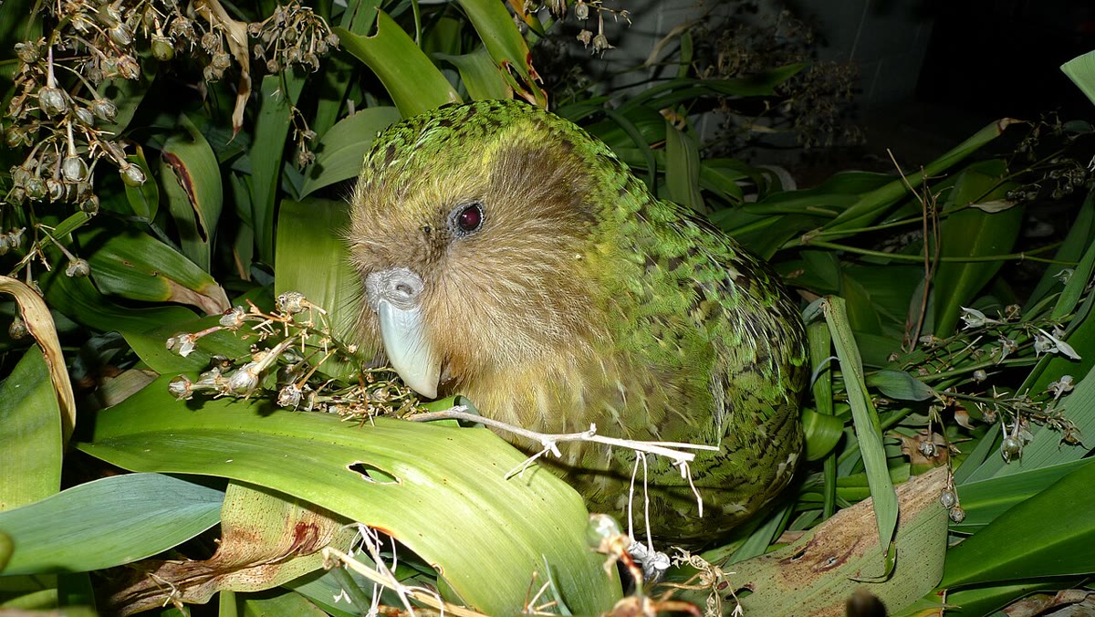
The kakapo: fifty-one birds in 1995, all moved to islands cleared of predators; every bird carries a transmitter, every nest is watched by camera, chicks are hand-reared when a mother fails, males are fed to bring them into breeding condition in the years the rimu trees fruit, and the pedigree is managed to keep the last Fiordland male’s rare genes in the population; every kakapo’s genome has been sequenced. Two hundred and fifty now, and a $N_{e}$ that the genomes put near a hundred. The whooping crane: fifteen birds in 1941, a single migratory flock, bred in captivity from eggs taken from wild nests, taught new migration routes behind ultralight aircraft, and now some eight hundred. The humpback whale: hunted to a few thousand, protected in 1966, and past a hundred thousand, an increase near $8\,\%$ a year that shows what a long-lived animal does when the single cause of its decline is removed. Each recovery cost tens of millions and decades; the arithmetic of the chapter says why the effort had to be spent before the numbers reached the vortex, and why it was cheaper than any later rescue would have been.

A seed vault in permafrost: duplicates of a million crop and wild-plant accessions, kept at -18\, C against the loss of the collections they came from — conservation as insurance, at the scale of a species’ genome. — A seed vault in permafrost: duplicates of a million crop and wild-plant accessions, kept at $-18\,{}^{\circ}\mathrm{C}$ against the loss of the collections they came from — conservation as insurance, at the scale of a species’ genome.

Remark 27.8 (The arithmetic of keeping)

Every chapter of this course has ended in a number, and this one ends in several: an effective size, an inbreeding coefficient rising by $1/2N_{e}$ a generation, an exponent $z$ that turns lost hectares into lost species, a probability of extinction over a century. They are crude — the census is uncertain, the variance is guessed, the model is a caricature — and they are what turns a sentiment about vanishing birds into a decision about which fifty hectares to buy and which eight animals to move. The biology is the same biology as the rest of the book: drift, selection, demography, behaviour, the dependence of a population on its habitat and of a habitat on its populations. What is new is only the urgency, and the fact that the experiment is being run once, without a control, on the species that are left.

27.4 Exercises

Exercise 27.1 ★

Define demographic stochasticity, environmental stochasticity and the Allee effect, and give one example of each from the chapter.

Solution

Solution of Exercise 27.1.

Demographic stochasticity: chance in the births, deaths and sexes of a few individuals — the kakapo at fifty-one, with more males than females. Environmental stochasticity: a bad year that hits every individual at once — a drought, a disease, a hard winter striking a population of a few hundred. Allee effect: per-capita growth falling at low density — the passenger pigeon, whose colonies could not breed once they had thinned, and whose remaining predators were no longer swamped.

Exercise 27.2 ★

What is the effective population size, and name three features of a real population that make it smaller than the census.

Solution

Solution of Exercise 27.2.

The size of an ideal population — constant, randomly mating, equal sexes, Poisson family sizes — that would lose heterozygosity at the same rate as the real one. Unequal numbers of breeding males and females; fluctuations in size, which weight the smallest generations; variance in family size above Poisson, with a few individuals producing most of the young (also non-random mating and overlapping generations).

Exercise 27.3 ★

State the species–area law. If $z = 0.25$ , what fraction of species does a habitat keep after losing half its area? Nine tenths? Ninety-nine hundredths?

Solution

Solution of Exercise 27.3.

$S = cA^{z}$ . Fraction kept $= (A'/A)^{z}$ : $0.5^{0.25} = 0.84$ ; $0.1^{0.25} = 0.56$ ; $0.01^{0.25} = 0.32$ — a hundredth of the area still keeps a third of the species, eventually.

Exercise 27.4 ★

Explain the 50/500 rule, and what each number protects against.

Solution

Solution of Exercise 27.4.

$N_{e} \ge 50$ keeps the rise of inbreeding below $1/100$ per generation, the rate at which animal breeders find depression tolerable: it guards against short-term loss of fitness. $N_{e} \ge 500$ balances the loss of variation by drift against its supply by mutation, so the population keeps the quantitative variation it needs to adapt: it guards the long term. Real populations need five to ten times these numbers in the census.

Exercise 27.5 ★★

A herd of 200 elephant seals has 8 breeding males and 120 breeding females. Compute $N_{e}$ and the loss of heterozygosity per generation. How many generations to lose a quarter of it?

Solution

Solution of Exercise 27.5.

$N_{e} = 4\times 8\times 120/128 = 30$ ; heterozygosity falls by $1/60 = 1.7\,\%$ a generation; a quarter lost when $(1 - 1/60)^{t} = 0.75$ , $t = \ln 0.75/\ln(59/60) = 17$ generations.

Exercise 27.6 ★★

A population numbered 1000, 1000, 20, 1000, 1000 in five successive generations. Compute $N_{e}$ over the span, and the heterozygosity retained, and compare with a constant 1000.

Solution

Solution of Exercise 27.6.

$1/N_{e} = \tfrac{1}{5}(4/1000 + 1/20) = 0.0108$ , $N_{e} = 93$ : one generation at twenty has made five generations behave like ninety-three. Heterozygosity retained $(1 - 1/186)^{5} = 0.973$ , against $(1 - 1/2000)^{5} = 0.9975$ for a constant thousand.

Exercise 27.7 ★★

Twenty-five Florida panthers with $N_{e} \approx 10$ : inbreeding accumulated in 5 generations? If fitness falls $5\,\%$ for every $10\,\%$ of $F$ , by how much has fitness fallen? What does adding eight unrelated females do to $F$ in the next generation?

Solution

Solution of Exercise 27.7.

$F = 1 - (1 - 1/20)^{5} = 0.23$ ; fitness down $5\times 2.3 = 11\,\%$ . Every offspring of a Texas female and a Florida male has $F = 0$ ; if the eight newcomers are two fifths of the breeding females, two fifths of the next generation are outbred and the mean $F$ falls to about $0.6\times 0.23 = 0.14$ in one generation — which is what the recovery showed.

Exercise 27.8 ★★

Yellowstone: 31 wolves released in 1995–96, about 100 in the park by 2003. Estimate $r$ ; how many would there be in 2020 if growth continued, and why did it not?

Solution

Solution of Exercise 27.8.

$r = \ln(100/31)/8 = 0.15\,\mathrm{yr}^{-1}$ . Continued to 2020: $100\,\mathrm{e}^{0.15\times 17} \approx 1200$ . The park held about a hundred: territories filled, elk declined, packs killed one another’s members, and mange and distemper spread — density dependence set in once the empty range was occupied.

Exercise 27.9 ★★

Classify by the IUCN criteria in the chapter: (a) a frog whose population fell $60\,\%$ in ten years; (b) a plant of 180 mature individuals; (c) a fish whose range is $3000\,\mathrm{km}^{2}$ ; (d) a bird of $30\,000$ individuals declining $10\,\%$ a decade.

Solution

Solution of Exercise 27.9.

(a) A $60\,\%$ decline in ten years exceeds $50\,\%$ : Endangered. (b) $180 < 250$ mature individuals: Critically Endangered. (c) Range $3000\,\mathrm{km}^{2}$ , below $5000\,$ : Endangered. (d) $30\,000$ individuals and a $10\,\%$ decline: neither threshold met — not threatened (at most Near Threatened, to be watched).

Exercise 27.10 ★★★

A population of $N$ pairs each producing, with probability $1/2$ , two surviving offspring and otherwise none (demographic stochasticity). Compute the probability that the whole population fails in one generation for $N = 2$ , $5$ , $10$ , $20$ , and comment on how demographic risk scales with $N$ .

Solution

Solution of Exercise 27.10.

All $N$ pairs fail with probability $(1/2)^{N}$ : $0.25$ , $0.031$ , $0.001$ , $10^{-6}$ . Demographic risk falls exponentially with $N$ and is negligible beyond a few dozen individuals; above that, the risk that remains is environmental, which does not fall so fast, because it strikes all individuals together.

Exercise 27.11 ★★★

The species–area law with $z = 0.25$ , and a forest cut into 10 equal isolated fragments. Compare the species expected in one fragment with a tenth of the original, and argue why the total across fragments is not simply the original — what determines whether the fragments together hold more or fewer species than the whole did?

Solution

Solution of Exercise 27.11.

One fragment of a tenth: $0.1^{0.25} = 0.56$ of the original species. Ten fragments hold between $0.56$ (if all hold the same species) and, in principle, more than the whole (if each held different species — impossible beyond the regional pool). Where they fall depends on turnover between fragments: different habitats in different fragments push the total up; species that need large areas, interior habitat, or that are lost from every fragment by the same edge effects push it down; and each fragment’s extinction debt is paid separately, so the long-run total is usually below the whole’s.

Exercise 27.12 ★★★

Why does adding a few migrants per generation ( $m N_{e} \approx 1$ ) largely stop the loss of variation in a small population, and what does it cost in local adaptation? Use the balance between drift, $1/2N_{e}$ , and the fraction of alleles replaced by migrants, $m$ , to argue.

Solution

Solution of Exercise 27.12.

Drift removes heterozygosity at rate $1/2N_{e}$ per generation; immigrants replace a fraction $m$ of the gene pool with alleles drawn from elsewhere. With $mN_{e} \approx 1$ , $m \approx 1/N_{e}$ , twice the rate of loss, so variation is replenished faster than it decays and the population stays close to the source in allele frequency ( $F_{ST} = 1/(1 + 4N_{e}m) \approx 0.2$ ). The cost: locally favoured alleles are diluted by $m$ per generation, so local adaptation survives only for traits whose selection coefficient exceeds about $1/N_{e}$ ; weakly selected local differences are swamped.

27.5 Problem: Fifty and Five Hundred

Problem 27.1

Weekend problem — a recovery programme in numbers: the effective size of a rescued parrot population and its inbreeding, a genetic rescue, the species a shrinking forest will keep, the growth of reintroduced wolves, and the categories and costs, ending on $N_{e}$ , the inbreeding after ten generations and the fraction of species kept

Data: a parrot population of 60 adults, 20 males and 40 females, all breeding; generation time $10\,\mathrm{yr}$ . Population history over the last five generations: 500, 100, 60, 51, 60. Inbreeding depression: fitness falls by $6\,\%$ for each $0.1\,$ of $F$ . Rescue: 10 unrelated birds added to 60. Forest: $2000\,\mathrm{km}^{2}$ reduced to $300\,\mathrm{km}^{2}$ , $z = 0.25$ ; species now 180. Wolves: 31 released, 100 after 8 years, carrying capacity in the park about 120. Cost: four million dollars a year for the parrots.

Part I — Effective size.

$N_{e}$ from the sex ratio of the current 60. Compare with the census.
Harmonic-mean $N_{e}$ over the five generations of history. Which generation dominates?
Inbreeding accumulated over those five generations, using the harmonic-mean $N_{e}$ (exact formula and linear approximation).
Fitness lost to that inbreeding.
Heterozygosity retained after the five generations, as a fraction of the original.
If the population is now held at 60 with the current sex ratio, what $F$ will it reach in ten more generations, and what fitness loss? How many years is that?

Part II — Rescue.

Ten unrelated birds join the 60. The fraction of alleles in the next generation from the newcomers is about $10/70$ ; the inbreeding coefficient of offspring with one native and one newcomer parent is $0$ . Estimate the population’s mean $F$ in the next generation if mating is random.
Explain why $F$ falls at once but heterozygosity rises only as the migrants’ alleles spread, and why a second rescue may be needed.
To reach $N_{e} = 500$ with an equal sex ratio, how many adults are needed? At $r = 0.05\,\mathrm{yr}^{-1}$ from 70 birds, how many years?
The programme removes eggs from poor mothers for hand-rearing, raising the mean number of fledged chicks per pair but equalising family sizes. Why does equalising family sizes raise $N_{e}$ above the census (toward $2N$ )?
The last male of a distinct southern lineage is sterile in the wild. Propose two interventions and their costs to the gene pool.
At four million dollars a year over the 40 years to reach $N_{e} = 500$ , total cost, and cost per bird added. Is that expensive? Against what?

Part III — Forest.

Fraction of species the forest will keep at $300\,\mathrm{km}^{2}$ ; expected number of species, and the extinction debt (species present now that will be lost).
If instead the $300\,\mathrm{km}^{2}$ were three isolated fragments of $100\,\mathrm{km}^{2}$ , species per fragment; total if the fragments held entirely different species; total if identical. What decides?
A corridor of $20\,\mathrm{km}^{2}$ joins the three fragments. Treat them as one area of $320\,\mathrm{km}^{2}$ : species expected. Compare with question 14’s identical-species case.
The forest’s largest predator needs $50\,\mathrm{km}^{2}$ per pair and an $N_{e}$ of 50 to persist. Can the whole $300\,\mathrm{km}^{2}$ hold it? Can a fragment? What does this say about area versus number of species as a criterion?
Estimate how long the extinction debt takes to be paid if the species lost have populations declining at $3\,\%$ a year from 200 to a quasi-extinction threshold of 10.
Why does the species–area law underestimate the loss when fragmentation adds edge effects, and overestimate it when the surrounding land is partly usable?

Part IV — Wolves and lists.

Wolves: $r$ from $31 \to 100$ in 8 years, and the doubling time.
Logistic growth toward $K = 120$ : population after 8 years under logistic rather than exponential growth, starting from 31 with the $r$ of question 19 (use $N(t) = K/[1 + (K/N_{0} - 1)\mathrm{e}^{-rt}]$ ). Which fits the observed 100 better, and what does that say about density dependence in the first years?
The elk numbered $17\,000$ in 1995 and $4000$ in 2015. Average annual rate of decline. How much of it can wolves eating $20$ elk each a year account for at 100 wolves?
Classify the parrot (60 mature individuals) and the pre-rescue forest predator by the IUCN criteria.
Passenger pigeon: five billion in 1800, extinct in 1914. If the decline was exponential from 1870, when there were still billions, to one bird in 1914, what annual rate does that imply? Why does the Allee effect make the last decades faster than exponential?
Explain in a paragraph why a PVA would have said the passenger pigeon was safe in 1850, and what it would have missed.
Summarise: the current $N_{e}$ (question 1), $F$ after ten more generations at 60 (question 6), and the fraction of species the shrunken forest keeps (question 13).

Solution

Solution of Problem 27.1.

1. $N_{e} = 4\times 20\times 40/60 = 53$ , against a census of 60. 2. $1/N_{e} = \tfrac{1}{5}(1/500 + 1/100 + 1/60 + 1/51 + 1/60) = 0.0130$ , $N_{e} = 77$ ; the bottleneck generations of 51 and 60 dominate, the 500 hardly counts. 3. $F = 1 - (1 - 1/154)^{5} = 0.032$ ; linear $5/154 = 0.032$ . 4. $6\times 0.32 = 1.9\,\%$ . 5. $(1 - 1/154)^{5} = 0.968$ : $96.8\,\%$ retained. 6. Ten generations at $N_{e} = 53$ : increment $1 - (1 - 1/107)^{10} = 0.090$ , total $F = 1 - 0.968\times 0.910 = 0.12$ ; fitness loss $6\times 1.2 = 7\,\%$ ; a century. 7. Native–native pairs are $(60/70)^{2} = 0.73$ of matings and their offspring keep $F \approx 0.03$ (plus a small increment); all others have $F = 0$ : mean $F \approx 0.73\times 0.035 = 0.026$ , a fall of a quarter in one generation. 8. $F$ is identity by descent within an individual, and any outbred offspring resets it to zero; heterozygosity is a property of allele frequencies, and the migrants’ alleles spread only as they are passed on. In a population still small, drift will remove them again within tens of generations, so rescue must be repeated or the population grown. 9. $N_{e} = N$ for equal sexes: 500 adults. From 70 at $r = 0.05$ : $\ln(500/70)/0.05 = 39$ years. 10. The ideal population has Poisson family sizes, variance equal to the mean of two; $N_{e} = 4N/(2 + V_{k})$ , so making every pair contribute equally ( $V_{k} = 0$ ) gives $N_{e} = 2N$ : no lineage is lost by the luck of the nest. 11. Collect and store his semen for artificial insemination, and use it on several unrelated females across years — the cost is that his alleles could come to dominate a small pool, so his share must be capped near $1/N_{e}$ ; or cryopreserve tissue for later cloning or gamete production, at the cost of delay and technical risk. Doing nothing loses the lineage’s alleles for good. 12. $160\,$ million dollars for some 430 birds: about $370\,000$ per bird. Expensive per parrot, cheap against a species — and less than a few kilometres of motorway, which is the comparison budgets actually make. 13. $(300/2000)^{0.25} = 0.62$ : about 112 species of 180 kept, an extinction debt of 68. 14. Each fragment $(100/2000)^{0.25}\times 180 = 85$ species. Entirely different: up to 255, impossible above the pool of 180; identical: 85. What decides is how different the fragments’ habitats are and how many species can persist in $100\,\mathrm{km}^{2}$ ; realistically between 85 and 112. 15. $(320/2000)^{0.25}\times 180 = 114$ , against 85 for three isolated identical fragments: the corridor lets recolonisation and gene flow make three small populations behave as one larger one. 16. $N_{e} = 50$ with equal sexes is 25 pairs: $1250\,\mathrm{km}^{2}$ . The whole $300\,\mathrm{km}^{2}$ holds six pairs, $N_{e} \approx 12$ ; a fragment, two. Neither suffices: the predator is lost whatever the species count, and protecting the area it needs protects everything smaller — an umbrella species. 17. $\ln(200/10)/0.03 = 100$ years: the debt is paid over a century, long after the forest was cut. 18. Edges strip interior habitat from every fragment, so the usable area is less than the mapped one and the loss is greater than the law predicts; a matrix of secondary growth or hedgerows that some species can use adds effective area and makes the loss smaller. 19. $r = \ln(100/31)/8 = 0.146\,\mathrm{yr}^{-1}$ ; doubling time $\ln 2/0.146 = 4.7$ years. 20. $N(8) = 120/[1 + (120/31 - 1)\mathrm{e}^{-1.17}] = 120/(1 + 2.87\times 0.31) = 63$ . The observed 100 is the exponential value itself — $r$ was fitted to those very two points — against the logistic 63: in the first years the wolves met no density dependence — empty territories and abundant elk. 21. $\ln(4000/17\,000)/20 = -0.072$ : $7\,\%$ a year. A hundred wolves taking $2000$ elk a year from a herd averaging $8000$ is a quarter a year — more than enough to drive the decline on its own, though hunting outside the park, drought and grizzly predation on calves shared it. 22. Sixty mature individuals, below 250: Critically Endangered. The predator at $N_{e} \approx 12$ (a few dozen animals): Critically Endangered as well. 23. From $3\times 10^{9}$ to $1$ in 44 years: $r = -\ln(3\times 10^{9})/44 = -0.50$ per year, halving every seventeen months. No harvest removes half of billions every year; the fall was slower at first and far faster at the end, because a colonial breeder below a threshold density stops reproducing while its predators are no longer swamped — the Allee effect turned a decline into a collapse. 24. In 1850 the population was in the billions, its measured growth rate positive and its variance small, and a viability analysis projects the dynamics it is given: it would have put the risk at zero. It would have missed the external forcing — railways and the telegraph that let hunters follow and empty every roost, forest clearance — and the Allee threshold in a colonial breeder, neither of which is in the demography of an abundant species; a PVA extrapolates, and the causes of extinction are usually new. 25. $N_{e} \approx 53$ today; $F \approx 0.12$ after ten more generations at 60 ( $7\,\%$ of fitness); the shrunken forest keeps about $62\,\%$ of its species.

Terms defined in this chapter

See all 479 terms in the glossary