High School Earth and Space Sciences · Grades 10–12

28Climate Change: Observations, Causes and Projections

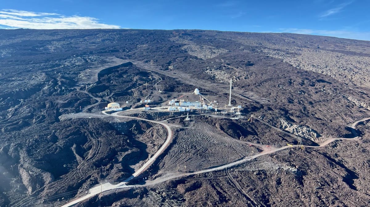
High on the northern slope of Mauna Loa, a volcano in the middle of the Pacific Ocean, a cluster of white buildings stands on bare lava, $3397\,\mathrm{m}$ above the sea. Up there, above the layer of air polluted by the island below and thousands of kilometres from any large city, the air is about as clean and well mixed as the atmosphere of the whole planet. Since March 1958, its carbon dioxide has been measured almost without a break. The record began as one chemist’s project; it has become the most famous curve in Earth science. This chapter reads that curve and the other records of the climate, explains how a change in the air changes the energy budget of the planet, how scientists decide what caused the warming they observe, and what they project for the decades to come.

The Mauna Loa Observatory, Hawaii, on old lava flows high on the north flank of the volcano. Photograph: Brian Vasel, NOAA (public domain).

You already know

The Earth receives energy from the Sun as light and loses the same amount on average to space as infrared radiation; the fraction of sunlight reflected is the albedo (Chapter 3). Greenhouse gases — water vapour, carbon dioxide, methane — absorb part of the infrared that the surface emits and send part of it back down; this greenhouse effect keeps the surface far warmer than it would otherwise be (the chemistry books, and Book 1, grade 9). Ice cores keep bubbles of ancient air and record the glacial cycles of the last 800 000 years (Chapter 27).

28.1 The records

The carbon dioxide content of the air at Mauna Loa: monthly means (line) and annual means (dots), in parts per million (ppm) of dry air. Data: NOAA Global Monitoring Laboratory and Scripps Institution of Oceanography.

Proposition 28.1 (The carbon dioxide record)

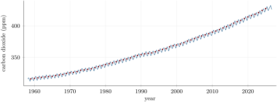
At Mauna Loa, the annual mean concentration of carbon dioxide rose from $316.0\,\mathrm{ppm}$ in 1959 to $427.4\,\mathrm{ppm}$ in 2025, and the rise is getting faster: the concentration grew by about $0.9\,\mathrm{ppm}$ per year in the 1960s and by about $2.6\,\mathrm{ppm}$ per year between 2015 and 2025. Every year the concentration also swings by about $7\,\mathrm{ppm}$ : it is highest in May and lowest in September.

Remark 28.2 (Why the curve has teeth)

The yearly swing is the breathing of the vegetation of the Northern Hemisphere, where most land plants are. In spring and summer, plants take up more carbon dioxide by photosynthesis than they and the soil release; in autumn and winter, decay and respiration win. The rise from year to year is a different story: it is the carbon of fossil fuels and of cleared forests accumulating in the air.

Proposition 28.3 (Higher than for at least two million years)

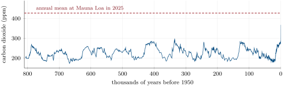
Over the last 800 000 years, the air bubbles of Antarctic ice record carbon dioxide concentrations between about $174\,\mathrm{ppm}$ , in the coldest glacial periods, and $299\,\mathrm{ppm}$ , in the warmest interglacials. Today’s value lies more than $100\,\mathrm{ppm}$ above the highest of them. The assessments state that the concentration in 2019 was higher than at any time in at least two million years (high confidence).

Carbon dioxide in Antarctic ice over 800 000 years: the glacial cycles move it between about 180 and 300\, ppm. The thin spike at the right-hand end is the youngest ice, which records the start of the present rise, up to the year 2001. Data: Bereiter and others (2015), NOAA Paleoclimatology. — Carbon dioxide in Antarctic ice over 800 000 years: the glacial cycles move it between about 180 and $300\,\mathrm{ppm}$ . The thin spike at the right-hand end is the youngest ice, which records the start of the present rise, up to the year 2001. Data: Bereiter and others (2015), NOAA Paleoclimatology.

Global mean surface temperature, as the difference from its average over 1951–1980. Data: NASA GISS Surface Temperature Analysis (GISTEMP v4).

Proposition 28.4 (Global warming observed)

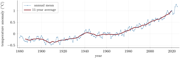
Each of the last four decades has been warmer than any decade before it since 1850. The global surface temperature of 2011–2020 was $1.09{}^{\circ}\mathrm{C}$ higher than that of 1850–1900 (very likely between 0.95 and $1.20{}^{\circ}\mathrm{C}$ ), with more warming over land ( $1.59{}^{\circ}\mathrm{C}$ ) than over the ocean ( $0.88{}^{\circ}\mathrm{C}$ ).

Proposition 28.5 (Sea level rises faster and faster)

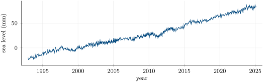
Global mean sea level rose by about $0.20\,\mathrm{m}$ between 1901 and 2018. The rate was about $1.3\,\mathrm{mm}$ per year from 1901 to 1971, $1.9\,\mathrm{mm}$ per year from 1971 to 2006 and $3.7\,\mathrm{mm}$ per year from 2006 to 2018 (high confidence). Satellites, measuring the height of the sea surface since 1993, find an average of $3.2\,\mathrm{mm}$ per year over 1993–2025. The sea rises because the warming ocean expands and because glaciers and ice sheets lose ice to it.

Global mean sea level measured from space, about every ten days (seasonal signal removed), relative to an arbitrary zero. Altimetry data are provided by NOAA Laboratory for Satellite Altimetry.

Figures as of 2025

The annual mean carbon dioxide concentration at Mauna Loa in 2025 was $427.35\,\mathrm{ppm}$ . In the NASA temperature record, the warmest year so far was 2024, at $1.28{}^{\circ}\mathrm{C}$ above the 1951–1980 average.

28.2 Radiative forcing

Definition 28.6 (Radiative forcing)

The radiative forcing of a change in the climate system — more greenhouse gas, more aerosol particles, a brighter Sun — is the change it causes in the net flow of energy entering the climate system at the top of the atmosphere, before the surface temperature has had time to respond. It is measured in watts per square metre ( $\mathrm{W}/\mathrm{m}^{2}$ ) of the Earth’s surface. A positive forcing makes the planet gain energy and warm; a negative forcing makes it lose energy and cool.

Remark 28.7 (Effective forcing)

The assessments use the effective radiative forcing, which also counts the fast adjustments of the atmosphere (of its clouds, for instance) that happen before the surface warms. All the forcings of this chapter are effective forcings.

Proposition 28.8 (The forcing since 1750)

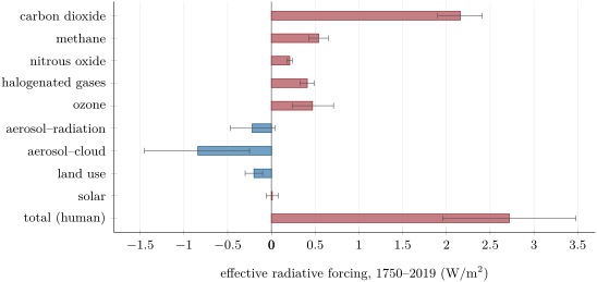
Human activities have produced a total radiative forcing of $2.72\,\mathrm{W}/\mathrm{m}^{2}$ in 2019 relative to 1750 (very likely between 1.96 and $3.48\,\mathrm{W}/\mathrm{m}^{2}$ ). The greenhouse gases contribute a positive forcing, led by carbon dioxide ( $2.16\,\mathrm{W}/\mathrm{m}^{2}$ ); aerosol particles, which reflect sunlight and brighten clouds, contribute a negative one (about $-1.06\,\mathrm{W}/\mathrm{m}^{2}$ in all). The change in the Sun’s brightness over the same period contributes only $0.01\,\mathrm{W}/\mathrm{m}^{2}$ .

The main effective radiative forcings from 1750 to 2019, with their very likely ranges (whiskers). Values: IPCC Sixth Assessment Report, Working Group I, Table 7.8.

Proposition 28.9 (Carbon dioxide: each doubling adds the same forcing)

To a good approximation, the forcing of carbon dioxide grows with the logarithm of its concentration: each doubling adds the same forcing, $F_{2\times} = 3.93\,\mathrm{W}/\mathrm{m}^{2}$ for a doubling from the concentration of 1750, $C_0 = 278\,\mathrm{ppm}$ . The forcing of a concentration $C$ is then

F = F_{2\times}\,\frac{\ln (C/C_0)}{\ln 2}.

Example 28.10 (Checking the law against the assessment)

In 2019 the concentration was $410\,\mathrm{ppm}$ . The law gives $F = 3.93 \times \ln(410/278)/\ln 2 = 3.93 \times 0.561 \approx 2.20\,\mathrm{W}/\mathrm{m}^{2}$ , within 2 % of the $2.16\,\mathrm{W}/\mathrm{m}^{2}$ that the assessment gives for carbon dioxide over 1750–2019.

Proposition 28.11 (Where the extra energy goes)

Because the forcing is positive, the climate system gains energy: about $0.79\,\mathrm{W}/\mathrm{m}^{2}$ on average over 2006–2018, up from $0.50\,\mathrm{W}/\mathrm{m}^{2}$ over 1971–2006 (high confidence). The ocean took 91 % of this energy; the land 5 %, the melting ice 3 % and the atmosphere only 1 %.

28.3 Feedbacks and climate sensitivity

When the surface warms, it radiates more energy to space, which tends to bring the planet back into balance. But the warming also changes other things — the water vapour in the air, the snow and ice on the ground, the clouds — and these changes alter the energy budget in their turn.

Definition 28.12 (Climate feedback)

A climate feedback is a change in the climate system, caused by a change in temperature, that alters the energy budget and so the temperature change itself. A positive feedback amplifies the initial change; a negative feedback damps it.

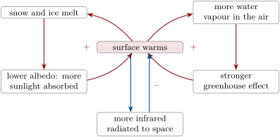
Example 28.13 (Three feedbacks)

Water vapour (positive). Warmer air holds more water vapour, a greenhouse gas, which adds to the warming.
Snow and ice (positive). Snow and ice reflect sunlight; when they melt, the darker land and sea beneath absorb more of it, and the warming grows.
Radiation to space (negative). A warmer surface and atmosphere radiate more infrared to space. This basic response always wins in the end: it is why the climate settles at a new, warmer balance instead of warming without limit.

Two positive feedbacks (red loops) amplify a warming; the extra infrared radiated by a warmer planet (blue) is a negative feedback that limits it.

Proposition 28.14 (Warming at equilibrium)

Once the climate has reached a new balance, the warming $\Delta T$ caused by a constant forcing $F$ is

\Delta T = \frac{F}{\lambda},

where $\lambda$ , the climate feedback parameter, is the extra energy the planet loses to space for each degree of warming. The assessments combine the radiation to space ( $3.22\,\mathrm{W}\,\mathrm{m}^{-2}\,{}^{\circ}\mathrm{C}^{-1}$ ) with the positive feedbacks of water vapour and the temperature profile ( $1.30$ ), of surface albedo ( $0.35$ ) and of clouds ( $0.42$ , in the same unit) into $\lambda \approx 1.16\,\mathrm{W}\,\mathrm{m}^{-2}\,{}^{\circ}\mathrm{C}^{-1}$ .

Partial proof. At the new balance the climate system again loses to space as much energy as it gains, so the extra loss due to the warming, $\lambda\,\Delta T$ , must make up for the forcing: $\lambda\,\Delta T = F$ . That the extra loss is proportional to $\Delta T$ is an approximation, good for warmings of a few degrees, and admitted here. ∎

Definition 28.15 (Equilibrium climate sensitivity)

The equilibrium climate sensitivity is the warming of the Earth’s surface, once a new balance is reached, after the concentration of carbon dioxide has been doubled from its 1750 level.

Proposition 28.16 (How sensitive is the climate?)

Combining all the lines of evidence — the physics of the feedbacks, the observed warming, past climates — the assessments give a best estimate of $3{}^{\circ}\mathrm{C}$ for the equilibrium climate sensitivity, likely between 2.5 and $4{}^{\circ}\mathrm{C}$ (high confidence), and very likely between 2 and $5{}^{\circ}\mathrm{C}$ .

28.4 Who is responsible?

Method 28.17 (Reading a statement of the assessments)

The international assessments of climate science grade every finding in a fixed vocabulary, printed in italics:

a likelihood, the probability of an outcome: virtually certain 99–100 %, extremely likely 95–100 %, very likely 90–100 %, likely 66–100 %, about as likely as not 33–66 %, unlikely 0–33 %, very unlikely 0–10 %;
a confidence, the strength of the evidence and the agreement behind a finding: very low, low, medium, high, very high.

A range written $[x \text{ to } y]$ is a very likely range: there is a 90 % chance that the true value lies inside it. To read a statement, identify the quantity, its best estimate, its range, and the likelihood or confidence attached.

Definition 28.18 (Attribution)

Attribution is the assessment of how much of an observed change is due to each of its possible causes, with the likelihood of the result.

Proposition 28.19 (Human influence)

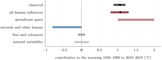
It is unequivocal that human influence has warmed the atmosphere, the ocean and the land. Between 1850–1900 and 2010–2019, the global surface warmed by about $1.06{}^{\circ}\mathrm{C}$ . Human activities caused a warming of $0.8{}^{\circ}\mathrm{C}$ to $1.3{}^{\circ}\mathrm{C}$ (likely range), best estimate $1.07{}^{\circ}\mathrm{C}$ : the well-mixed greenhouse gases likely warmed the surface by 1.0 to $2.0{}^{\circ}\mathrm{C}$ , and the other human influences, mainly aerosols, likely cooled it by 0 to $0.8{}^{\circ}\mathrm{C}$ . The Sun and volcanoes changed it by only $-0.1$ to $+0.1{}^{\circ}\mathrm{C}$ , and the natural fluctuations of the climate by $-0.2$ to $+0.2{}^{\circ}\mathrm{C}$ .

What caused the observed warming: likely ranges of each contribution, with the best estimates where the assessment gives one (dots); for the observed warming, its very likely range. Values: IPCC Sixth Assessment Report, Working Group I, Summary for Policymakers, A.1.3.

28.5 Scenarios and projections

Definition 28.20 (Scenario and projection)

An emission scenario is a consistent story of how the emissions of greenhouse gases and aerosols might evolve in the future. A projection is the response of the climate computed by models for a given scenario. A projection is not a forecast: it says what would happen if the scenario came true.

Proposition 28.21 (Projected warming and sea-level rise)

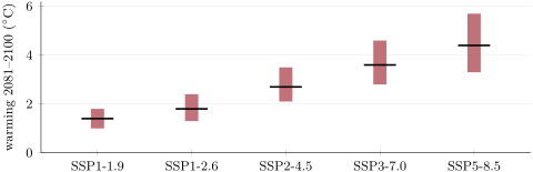
The assessments use five main scenarios, from very low emissions (SSP1-1.9) to very high emissions (SSP5-8.5). For 2081–2100, compared with 1850–1900, they project the warmings below (best estimates and very likely ranges, in ${}^{\circ}\mathrm{C}$ ), and, by 2100, the likely rises of global mean sea level relative to 1995–2014. Under every scenario the sea keeps rising through the century (virtually certain). The last time the global surface stayed $2.5{}^{\circ}\mathrm{C}$ or more above 1850–1900 was over three million years ago (medium confidence).

scenario	emissions	warming 2081–2100 ( ${}^{\circ}\mathrm{C}$ )	sea-level rise by 2100 (m)
SSP1-1.9	very low	1.4 (1.0 to 1.8)	0.28 to 0.55
SSP1-2.6	low	1.8 (1.3 to 2.4)	0.32 to 0.62
SSP2-4.5	intermediate	2.7 (2.1 to 3.5)	0.44 to 0.76
SSP3-7.0	high	3.6 (2.8 to 4.6)	—
SSP5-8.5	very high	4.4 (3.3 to 5.7)	0.63 to 1.01

Projected warming at the end of the century for the five scenarios: very likely range (bar) and best estimate (black line). Values: IPCC Sixth Assessment Report, Working Group I, Table SPM.1.

Remark 28.22 (What this chapter does not say)

Which scenario the world will follow depends on future emissions, that is, on decisions that are not questions of physics. The physical science says how the climate responds to each one; the choice among them belongs to societies, and its costs and benefits are studied by other sciences.

History — A curve that started as a chemist’s project

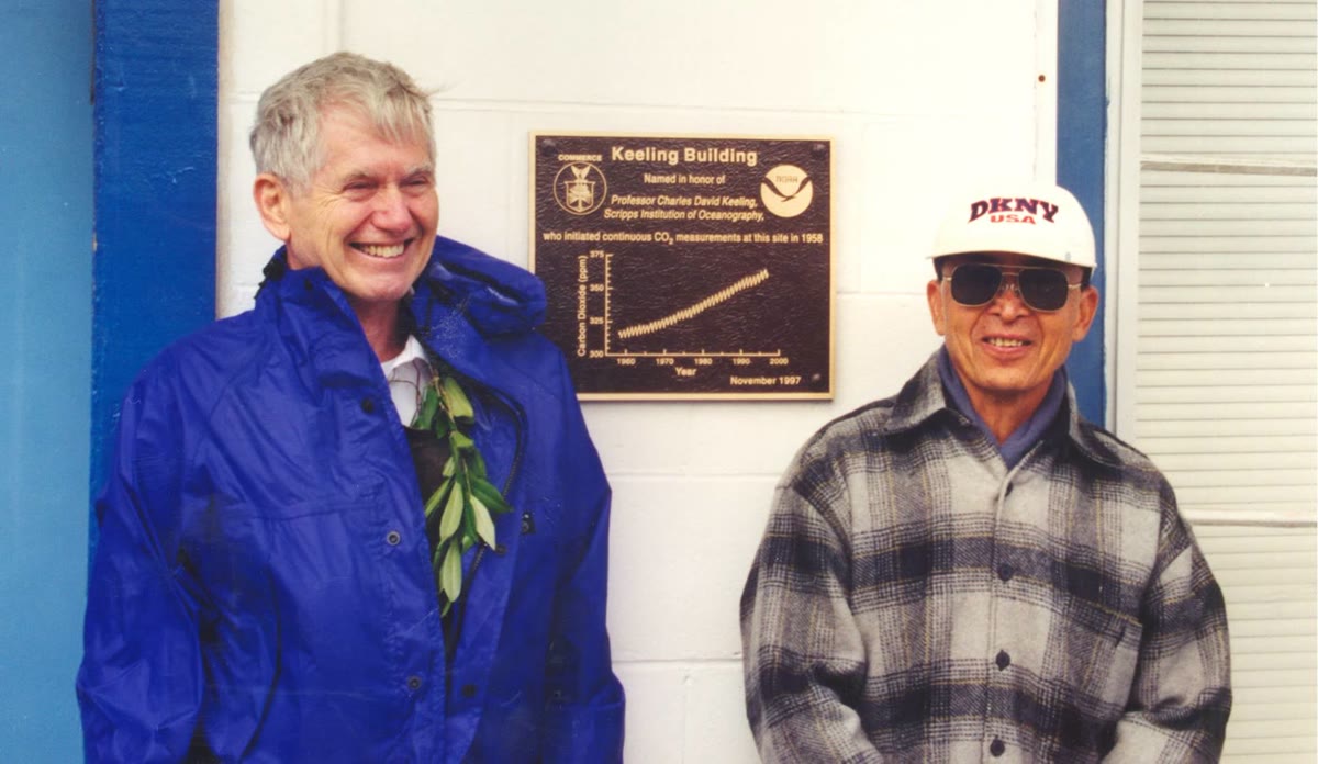
In March 1958 the chemist Charles David Keeling, of the Scripps Institution of Oceanography, began measuring the carbon dioxide of the air at Mauna Loa with an instrument precise enough to see changes of a fraction of a part per million. Within a few years his record showed both the yearly breathing of the vegetation and a steady rise. The measurements, continued since by Scripps and by the US weather and ocean agency, are the longest direct record of the composition of the atmosphere.

Charles David Keeling (left) and John Chin at the Mauna Loa Observatory in 1997, beside the plaque that names a building after Keeling. Photograph: John Miller, NOAA (public domain).

28.6 Exercises

Exercise 28.1 ★

What is the radiative forcing of a change in the climate system? In which unit is it measured, and what does its sign mean?

Solution

Solution of Exercise 28.1.

The change it causes in the net flow of energy entering the climate system at the top of the atmosphere, before the surface temperature responds; measured in $\mathrm{W}/\mathrm{m}^{2}$ . Positive: the planet gains energy and warms; negative: it loses energy and cools.

Exercise 28.2 ★

In which month of the year is the carbon dioxide concentration at Mauna Loa highest, and in which is it lowest? Explain the yearly swing.

Solution

Solution of Exercise 28.2.

Highest in May, lowest in September. In spring and summer the vegetation of the Northern Hemisphere, where most land plants grow, takes up more carbon dioxide by photosynthesis than plants and soils release; in autumn and winter decay and respiration dominate and the concentration rises again.

Exercise 28.3 ★

In the vocabulary of the assessments, what probability does very likely mean? And likely? What does a range written $[0.95 \text{ to } 1.20]$ mean?

Solution

Solution of Exercise 28.3.

Very likely: a probability of 90 to 100 %; likely: 66 to 100 %. $[0.95 \text{ to } 1.20]$ is a very likely range: a 90 % chance that the true value lies between 0.95 and 1.20.

Exercise 28.4 ★

Of the extra energy that the climate system has gained in recent decades, what share went into the ocean? Why does this explain why sea level rises even without melting ice?

Solution

Solution of Exercise 28.4.

91 %. Water expands when it warms: a warmer ocean occupies more volume, so its surface rises even if no water is added (melting land ice adds water on top of this).

Exercise 28.5 ★

Give two positive climate feedbacks and the negative response that limits the warming. Explain each in one sentence.

Solution

Solution of Exercise 28.5.

Water vapour: warmer air holds more water vapour, a greenhouse gas, which adds to the warming. Snow and ice: melting uncovers darker surfaces, which absorb more sunlight. The negative response: a warmer planet radiates more infrared to space, which brings it back to balance.

Exercise 28.6 ★★

The annual mean concentration of carbon dioxide at Mauna Loa was $315.98\,\mathrm{ppm}$ in 1959 and $427.35\,\mathrm{ppm}$ in 2025. By how many ppm, and by what percentage, did it increase? What was the average growth per year over the whole period?

Solution

Solution of Exercise 28.6.

$427.35 - 315.98 = 111.37\,\mathrm{ppm}$ ; $111.37/315.98 \approx 0.352$ , an increase of about 35 %. Over 66 years: $111.37/66 \approx 1.7\,\mathrm{ppm}$ per year on average.

Exercise 28.7 ★★

Use the logarithmic law of the chapter, with $F_{2\times} = 3.93\,\mathrm{W}/\mathrm{m}^{2}$ and $C_0 = 278\,\mathrm{ppm}$ , to compute the forcing of carbon dioxide at $427.35\,\mathrm{ppm}$ , the 2025 annual mean.

Solution

Solution of Exercise 28.7.

$F = 3.93 \times \ln(427.35/278)/\ln 2 = 3.93 \times 0.4300/0.6931 \approx 2.44\,\mathrm{W}/\mathrm{m}^{2}$ .

Exercise 28.8 ★★

At $3.7\,\mathrm{mm}$ per year, the rate of 2006–2018, how much would sea level rise in 30 years? How many times faster is this rate than that of 1901–1971, $1.3\,\mathrm{mm}$ per year?

Solution

Solution of Exercise 28.8.

$3.7 \times 30 = 111\,\mathrm{mm}$ , about $11\,\mathrm{cm}$ . $3.7/1.3 \approx 2.8$ : almost three times faster.

Exercise 28.9 ★★

Using $\Delta T = F/\lambda$ with $\lambda = 1.16\,\mathrm{W}\,\mathrm{m}^{-2}\,{}^{\circ}\mathrm{C}^{-1}$ , compute the equilibrium warming that the total human forcing of 2019, $2.72\,\mathrm{W}/\mathrm{m}^{2}$ , would produce. The observed human-caused warming is only about $1.07{}^{\circ}\mathrm{C}$ . Give the main reason for the difference.

Solution

Solution of Exercise 28.9.

$\Delta T = 2.72/1.16 \approx 2.3{}^{\circ}\mathrm{C}$ . The climate is not at equilibrium: the ocean, which takes up about 90 % of the extra energy, warms slowly, so the surface has not yet caught up with the forcing (the system still gains about $0.8\,\mathrm{W}/\mathrm{m}^{2}$ ).

Exercise 28.10 ★★

The Sun and volcanoes changed the global temperature between 1850–1900 and 2010–2019 by $-0.1$ to $+0.1{}^{\circ}\mathrm{C}$ , while the observed warming was about $1.06{}^{\circ}\mathrm{C}$ . What can you conclude? Which other natural cause must also be ruled out, and what does the assessment say about it?

Solution

Solution of Exercise 28.10.

The Sun and volcanoes explain at most $0.1{}^{\circ}\mathrm{C}$ of a $1.06{}^{\circ}\mathrm{C}$ warming: they cannot be its cause. The other natural cause is the internal variability of the climate (its natural fluctuations, such as exchanges of heat between ocean and atmosphere); the assessment puts its contribution at $-0.2$ to $+0.2{}^{\circ}\mathrm{C}$ , also far too small.

Exercise 28.11 ★★

Using the table of projections, under which scenarios is the warming of 2081–2100 very likely to stay below $2{}^{\circ}\mathrm{C}$ ? Under which is it very likely to exceed $2{}^{\circ}\mathrm{C}$ ?

Solution

Solution of Exercise 28.11.

Very likely below $2{}^{\circ}\mathrm{C}$ : only SSP1-1.9 (very likely range 1.0 to 1.8). Very likely above: SSP2-4.5 (2.1 to 3.5), SSP3-7.0 (2.8 to 4.6) and SSP5-8.5 (3.3 to 5.7). For SSP1-2.6 (1.3 to 2.4) neither is very likely.

Exercise 28.12 ★★★

Aerosols produced a forcing of about $-0.22$ and $-0.84\,\mathrm{W}/\mathrm{m}^{2}$ (through sunlight and through clouds). If all aerosols were removed from the air while everything else stayed as in 2019, what would the total human forcing become? By how much would the equilibrium warming increase, with $\lambda = 1.16\,\mathrm{W}\,\mathrm{m}^{-2}\,{}^{\circ}\mathrm{C}^{-1}$ ?

Solution

Solution of Exercise 28.12.

The aerosol forcing is $-0.22 - 0.84 = -1.06\,\mathrm{W}/\mathrm{m}^{2}$ ; without it the total becomes $2.72 + 1.06 = 3.78\,\mathrm{W}/\mathrm{m}^{2}$ . The equilibrium warming increases by $1.06/1.16 \approx 0.9{}^{\circ}\mathrm{C}$ .

Exercise 28.13 ★★★

Show, from the logarithmic law, that going from $278\,\mathrm{ppm}$ to $556\,\mathrm{ppm}$ and going from $556\,\mathrm{ppm}$ to $1112\,\mathrm{ppm}$ add the same forcing. What is the total forcing at $1112\,\mathrm{ppm}$ ?

Solution

Solution of Exercise 28.13.

Since $\ln(2C) - \ln C = \ln 2$ whatever $C$ ,

F(556) - F(278) = \frac{3.93\,\ln 2}{\ln 2} = 3.93\,\mathrm{W}/\mathrm{m}^{2}, \qquad F(1112) - F(556) = \frac{3.93\,\ln 2}{\ln 2} = 3.93\,\mathrm{W}/\mathrm{m}^{2}:

the same forcing for each doubling. Total at $1112\,\mathrm{ppm}$ : $2 \times 3.93 = 7.86\,\mathrm{W}/\mathrm{m}^{2}$ .

Exercise 28.14 ★★★

Differentiate the logarithmic law with respect to $C$ . How much forcing does one extra ppm of carbon dioxide add at $280\,\mathrm{ppm}$ , and how much at $420\,\mathrm{ppm}$ ? Comment.

Solution

Solution of Exercise 28.14.

$\dfrac{\dd F}{\dd C} = \dfrac{F_{2\times}}{C \ln 2}$ . At $280\,\mathrm{ppm}$ : $3.93/(280 \times 0.6931) \approx 0.0202\,\mathrm{W}/\mathrm{m}^{2}$ per ppm; at $420\,\mathrm{ppm}$ : $\approx 0.0135\,\mathrm{W}/\mathrm{m}^{2}$ per ppm. Each extra ppm adds less forcing as the concentration grows (1.5 times less at 420 than at 280), but the concentration keeps rising, so the forcing still grows.

Exercise 28.15 ★★★

Without any feedback except the extra radiation to space, $\lambda_0 = 3.22\,\mathrm{W}\,\mathrm{m}^{-2}\,{}^{\circ}\mathrm{C}^{-1}$ . Compute the warming for a doubling of carbon dioxide ( $F_{2\times} = 3.93\,\mathrm{W}/\mathrm{m}^{2}$ ) with $\lambda_0$ , then with $\lambda = 1.16\,\mathrm{W}\,\mathrm{m}^{-2}\,{}^{\circ}\mathrm{C}^{-1}$ . By what factor do the feedbacks amplify the warming?

Solution

Solution of Exercise 28.15.

$3.93/3.22 \approx 1.2{}^{\circ}\mathrm{C}$ without feedbacks; $3.93/1.16 \approx 3.4{}^{\circ}\mathrm{C}$ with them. Amplification factor: $3.22/1.16 \approx 2.8$ .

28.7 Problem: The Keeling Curve by the Numbers

Problem 28.1

Weekend problem — from the yearly breathing of the vegetation to the year a doubling would be reached

A student downloads the Mauna Loa record and works through it with a spreadsheet. Over 2015–2024, the monthly concentration lies on average $3.37\,\mathrm{ppm}$ above the smoothed trend in May and $3.51\,\mathrm{ppm}$ below it in September. The annual means are $316.91\,\mathrm{ppm}$ in 1960, $325.68\,\mathrm{ppm}$ in 1970, $401.01\,\mathrm{ppm}$ in 2015 and $427.35\,\mathrm{ppm}$ in 2025. The concentration of 1750 was $278\,\mathrm{ppm}$ . Use the logarithmic law with $F_{2\times} = 3.93\,\mathrm{W}/\mathrm{m}^{2}$ .

Part I — The breathing of the vegetation.

What is the peak-to-trough amplitude of the yearly cycle?
Explain why the concentration is highest in May and lowest in September.
The cycle is much weaker in the air of the Southern Hemisphere. Suggest why.
Why was the observatory built $3397\,\mathrm{m}$ high, on a volcano in the middle of the Pacific?

Part II — The trend.

Compute the average growth, in ppm per year, over 1960–1970.
Compute it over 2015–2025.
By what factor has the growth rate increased?
By what percentage did the concentration rise between 1750 and 2025?
The ice cores never show more than about $300\,\mathrm{ppm}$ over the last 800 000 years. By how many ppm does the 2025 value exceed this?

Part III — The forcing.

Compute the forcing of carbon dioxide in 2025.
Compute it in 1960, and the increase of the forcing between 1960 and 2025.
What concentration would add $1\,\mathrm{W}/\mathrm{m}^{2}$ to the forcing of 2025?
At the growth rate of 2015–2025, how many years would that take?

Part IV — The doubling.

What is the concentration of a doubling of the 1750 value? What forcing does it produce?
With the best estimate of the equilibrium climate sensitivity, what equilibrium warming would it cause? Give the likely range.
What feedback parameter $\lambda$ does a sensitivity of $3{}^{\circ}\mathrm{C}$ imply? Compare it with the value $1.16\,\mathrm{W}\,\mathrm{m}^{-2}\,{}^{\circ}\mathrm{C}^{-1}$ obtained by adding up the feedbacks.
Why would the surface not reach this warming on the day the doubling is reached?
Why is a calculation that simply prolongs today’s growth rate a scenario, and not a projection of the kind the assessments make?
If the growth rate of 2015–2025 stayed the same, in what year would the doubling of the 1750 concentration be reached?

Solution

Solution of Problem 28.1.

1. $3.37 + 3.51 = 6.88\,\mathrm{ppm}$ , about $7\,\mathrm{ppm}$ .

2. From spring to late summer, the plants of the Northern Hemisphere draw carbon dioxide out of the air by photosynthesis faster than respiration and decay return it: the concentration falls until September. In autumn and winter the balance reverses, and the concentration climbs back to its May maximum.

3. The Southern Hemisphere has much less land, and so much less vegetation, than the Northern; most of its surface is ocean.

4. High up, it lies above the layer of polluted air near the ground; far from continents and cities, the air it samples is well mixed and represents the whole atmosphere, not a local source.

5. $(325.68 - 316.91)/10 \approx 0.88\,\mathrm{ppm}$ per year.

6. $(427.35 - 401.01)/10 \approx 2.63\,\mathrm{ppm}$ per year.

7. $2.634/0.877 \approx 3.0$ : the growth rate has tripled.

8. $(427.35 - 278)/278 \approx 0.537$ : about 54 %.

9. $427.35 - 300 \approx 127\,\mathrm{ppm}$ .

10. $F = 3.93 \times \ln(427.35/278)/\ln 2 \approx 2.44\,\mathrm{W}/\mathrm{m}^{2}$ .

11. $F(316.91) = 3.93 \times \ln(316.91/278)/\ln 2 \approx 0.74\,\mathrm{W}/\mathrm{m}^{2}$ ; increase $2.44 - 0.74 \approx 1.70\,\mathrm{W}/\mathrm{m}^{2}$ .

12. One more $\mathrm{W}/\mathrm{m}^{2}$ multiplies the concentration by $2^{1/3.93} \approx 1.193$ : $427.35 \times 1.193 \approx 510\,\mathrm{ppm}$ .

13. $(509.8 - 427.35)/2.634 \approx 31$ years.

14. $2 \times 278 = 556\,\mathrm{ppm}$ ; forcing $F_{2\times} = 3.93\,\mathrm{W}/\mathrm{m}^{2}$ .

15. By definition of the sensitivity, $3{}^{\circ}\mathrm{C}$ (likely 2.5 to $4{}^{\circ}\mathrm{C}$ ).

16. $\lambda = 3.93/3 \approx 1.31\,\mathrm{W}\,\mathrm{m}^{-2}\,{}^{\circ}\mathrm{C}^{-1}$ . The sum of the feedbacks, $1.16\,\mathrm{W}\,\mathrm{m}^{-2}\,{}^{\circ}\mathrm{C}^{-1}$ , gives $3.93/1.16 \approx 3.4{}^{\circ}\mathrm{C}$ , a little more; the assessed best estimate combines this physics with the observed warming and past climates, and both values lie in the likely range.

17. The ocean stores most of the extra energy and warms slowly: the surface reaches its equilibrium warming only after decades to centuries.

18. It assumes one story of future emissions (the growth of the last ten years kept forever): that is a scenario. A projection computes the response of the climate and of the carbon cycle to a scenario of emissions with physical models, and gives ranges and likelihoods.

19. $(556 - 427.35)/2.634 \approx 48.8$ years after 2025: about 2074.

Terms defined in this chapter

See all 957 terms in the glossary