12Plate Kinematics on a Sphere

Two satellite-positioning stations have been recording their positions every day for more than a quarter of a century: one in Reykjavik, in the west of Iceland, the other near Stavanger, on the west coast of Norway. The straight line between them, $1546\,\mathrm{km}$ long, grows by $17.5\,\mathrm{mm}$ every year, nearly two centimetres. Nothing on the ground shows it, yet the floor of the North Atlantic between the two stations records the same widening over millions of years: lava erupted at the Mid-Atlantic Ridge took on the direction of the Earth’s magnetic field as it cooled, and the field has reversed many times, so that the ocean floor carries a striped record of its own growth. This chapter turns the plates of the school years into rigid caps on a sphere, describes their motions with the geometry of rotations, and shows how the geological record and the satellites measure the same motions.

You already know

On a sphere, a great circle is the intersection with a plane through the centre, a small circle with any other plane; the cosine rule gives the angular distance between two points from their latitudes and longitudes, and the azimuth of a direction is counted from north through east (Chapter 1). A rigid body turning about a fixed axis has an angular velocity (physics). The lithosphere is broken into plates that move relative to one another at a few centimetres a year, and the ocean floor carries magnetic stripes that record the reversals of the Earth’s magnetic field (Book 2, grade 11).

12.1 Rigid plates on a sphere

A plate covers a large part of the sphere: the Eurasian plate stretches from the middle of the Atlantic to eastern Siberia. Its motion cannot be described by a velocity, as the motion of a car can; it must be described by a rotation.

Definition 12.1 (Rigid plate)

A rigid plate is a region of the lithosphere whose interior does not deform measurably: the distance between any two of its points stays constant. The relative motion of two plates is taken up along their common boundary, a narrow zone of faults, earthquakes and volcanoes.

No plate is perfectly rigid: the boundaries are zones tens to hundreds of kilometres wide, and the interiors deform slowly. The hypothesis is that these departures are small beside the relative motions; it is tested by the consistency of every result of this chapter.

A rigid plate on the surface of a sphere moves without changing the distance between any two of its points, and the centre of the Earth does not move. Such a motion is described by a $3\times3$ matrix $R$ that keeps lengths, an orthogonal matrix ($R^{\mathsf T}R = I$), and that keeps the orientation of space, so that $\det R = 1$: a point at the position vector $\vec r$ goes to $R\vec r$.

Theorem 12.2 (Euler’s rotation theorem)

Every displacement of a rigid plate on the sphere is a rotation about an axis through the centre of the Earth: there is a unit vector $\vec n$ with $R\vec n = \vec n$, and the plate turns about $\vec n$ by some angle.

Over an interval of time short enough for the motion not to change, the rotation proceeds at a steady rate, and the motion of one plate relative to another is an angular velocity about a fixed axis.

Definition 12.3 (Euler pole; Euler vector)

The motion of a plate B relative to a plate A is a rotation about an axis through the centre of the Earth. The Euler pole of the pair is the point where this axis meets the surface, chosen so that the rotation is anticlockwise seen from above it; the antipodal point is the opposite pole. The Euler vector $\vec\omega_{BA}$ is the angular velocity of B relative to A: it points from the centre of the Earth towards the Euler pole, and its length $\omega$ is the rate of rotation.

An Euler vector is given by the latitude and longitude of its pole and its rate, usually in degrees per million years. The motion of the Eurasian plate relative to the North American plate, averaged over the last $3.16\,\mathrm{Myr}$ from 453 spreading rates measured on the ridges between them, has its pole at $61.8{}^{\circ}$ N, $139.6{}^{\circ}$ E, in eastern Siberia, and the rate $0.210{}^{\circ}/\mathrm{Myr}$. In radians per year,

a full turn in $1714\,\mathrm{Myr}$.

12.2 Relative velocities

Theorem 12.4 (Velocity on a rotating plate)

If plate B turns relative to plate A with the Euler vector $\vec\omega$, a point of B at the position vector $\vec r$ (from the centre of the Earth) moves relative to A with the velocity

$$\vec v = \vec\omega\times\vec r .$$

The angle $\Delta$ is the angular distance between the Euler pole and the point, which the cosine rule gives from latitudes and longitudes.

Proposition 12.5 (Speed and direction of relative motion)

Let the Euler pole be at latitude $\varphi_p$ and longitude $\lambda_p$, and the point at $\varphi$ and $\lambda$. Then

1. the angular distance $\Delta$ from the pole to the point satisfies $\cos\Delta = \sin\varphi_p\sin\varphi + \cos\varphi_p\cos\varphi \cos(\lambda - \lambda_p)$;
2. the relative speed is $v = \omega R\sin\Delta$: zero at the pole, largest, $\omega R$, on the great circle $90{}^{\circ}$ from it;
3. the direction of motion is perpendicular to the great circle that joins the point to the pole: its azimuth is that of the pole, as seen from the point, plus $90{}^{\circ}$.

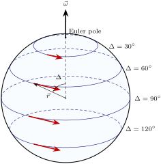
The speed of relative motion therefore changes along a plate boundary even when the two plates are perfectly rigid, and the direction of motion turns with it. Two consequences shape every plate boundary map.

Proposition 12.6 (Transforms follow small circles)

A transform fault, along which two plates slide past each other without opening or closing, lies on a small circle about the Euler pole of the two plates. The direction of spreading at a ridge, and of convergence at a subduction zone, is along the small circles too.

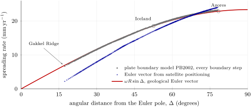
The Mid-Atlantic Ridge between Eurasia and North America is a staircase of ridge segments offset by transform faults; the transforms trend close to the azimuths the Euler vector predicts, and their trend is one of the data used to locate the pole. The spreading rate along the same boundary grows with the angular distance from the pole: $11\text{ to }12\,\mathrm{mm}\,\mathrm{yr}^{-1}$ on the Gakkel Ridge in the Arctic Ocean, near the pole, and $23\,\mathrm{mm}\,\mathrm{yr}^{-1}$ just north of the Azores, $78{}^{\circ}$ from it. The figure below compares the rates the Euler vector predicts all along the boundary with those of an independent plate model.

Method 12.7 (The velocity at a point)

1. Convert the rate of the Euler vector to radians per year and compute $\omega R$, in $\mathrm{mm}\,\mathrm{yr}^{-1}$ with $R = 6371\,\mathrm{km}$.
2. Compute the angular distance $\Delta$ from the pole to the point with the cosine rule; the speed is $\omega R\sin\Delta$.
3. Compute the azimuth $\beta$ of the pole as seen from the point, with $\tan\beta = \sin(\lambda_p - \lambda)\cos\varphi_p / \bigl(\cos\varphi\sin\varphi_p - \sin\varphi\cos\varphi_p \cos(\lambda_p - \lambda)\bigr)$ and the quadrant of the numerator and denominator; the motion is towards $\beta + 90{}^{\circ}$.
4. Check the sense: the motion is the one of the second plate relative to the first. Exchanging the plates reverses it.

Example 12.8 (Eurasia moves away from North America in Iceland)

Take the middle of Iceland at $64.5{}^{\circ}$ N, $18{}^{\circ}$ W, and the Euler vector of Eurasia relative to North America above. Then $\omega R = 3.665 \times 10^{-9}\times6.371 \times 10^{9}\,\mathrm{mm} = 23.35\,\mathrm{mm}\,\mathrm{yr}^{-1}$, and

$$\cos\Delta = \sin61.8{}^{\circ}\sin64.5{}^{\circ} + \cos61.8{}^{\circ}\cos64.5{}^{\circ}\cos(-18{}^{\circ} - 139.6{}^{\circ}) = 0.60736,$$

so $\Delta = 52.60{}^{\circ}$ and $v = 23.35\sin52.60{}^{\circ} = 18.55\,\mathrm{mm}\,\mathrm{yr}^{-1}$. The pole is seen at the azimuth $\beta = 13.1{}^{\circ}$, a little east of north, over the Arctic; Eurasia moves towards $103.1{}^{\circ}$, east-south-east, that is $18.07\,\mathrm{mm}\,\mathrm{yr}^{-1}$ to the east and $4.20\,\mathrm{mm}\,\mathrm{yr}^{-1}$ to the south.

12.3 Combining motions; triple junctions

Relative velocities add like the velocities of mechanics: if B moves relative to A and C relative to B, then C moves relative to A with the sum of the two velocities.

Proposition 12.9 (Euler vectors add)

For three plates A, B, C,

$$\vec\omega_{CA} = \vec\omega_{CB} + \vec\omega_{BA}, \qquad \vec\omega_{AB} = -\vec\omega_{BA}.$$

To add Euler vectors, write each in Cartesian components, $\omega(\cos\varphi_p \cos\lambda_p, \cos\varphi_p\sin\lambda_p, \sin\varphi_p)$, add the components, and convert back to a pole and a rate. Poles cannot be added; Euler vectors can. The relation is a powerful constraint. The motion of the Nubian plate (Africa) relative to Eurasia is slow, and the geological record gives few direct measures of it: between the Azores and Gibraltar, the only ones are the azimuths of a single transform, the Gloria fault. It follows instead from the two well-measured spreading motions across the Atlantic: with $\vec\omega_{\mathrm{NB\,NA}}$ (pole $79.2{}^{\circ}$ N, $40.2{}^{\circ}$ E, $0.233{}^{\circ}/\mathrm{Myr}$) and $\vec\omega_{\mathrm{EU\,NA}}$ above, $\vec\omega_{\mathrm{NB\,EU}} = \vec\omega_{\mathrm{NB\,NA}} - \vec\omega_{\mathrm{EU\,NA}}$ has its pole at $20.9{}^{\circ}$ N, $18.3{}^{\circ}$ W, off West Africa, and the rate $0.123{}^{\circ}/\mathrm{Myr}$ (Exercise 12.7).

Definition 12.10 (Triple junction; stable triple junction)

A triple junction is a point where three plates meet, and with them three plate boundaries, each a ridge (R), a trench (T) or a transform fault (F). A triple junction is stable if, as the plates move, it keeps the same geometry: the same three kinds of boundary meeting at the same angles.

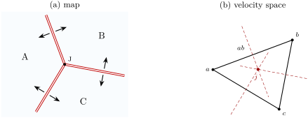
Each boundary allows the junction to move only in certain ways without changing its geometry. A symmetric ridge stays midway between its two plates; a transform keeps its trend whatever the junction does along it; a trench is fixed to its overriding plate. The question is whether one motion of the junction satisfies all three boundaries at once. It is answered in velocity space: a diagram in which each plate is a point whose position vector is the plate’s velocity at the junction, relative to any one plate, so that the side joining two points is the relative velocity of the two plates.

Proposition 12.11 (Ridge–ridge–ridge junctions are stable)

A junction of three ridges, each spreading symmetrically and perpendicular to its axis, is stable whatever the relative velocities of the three plates.

McKenzie and Morgan, who introduced the distinction between stable and unstable junctions in 1969, analysed the combinations in this way. A transform allows the junction to move only along itself, that is, along the line through the points of its two plates: a junction of three transforms is therefore never stable, since the three lines through the sides of a triangle have no common point. For the other kinds, stability places conditions on the orientations of the boundaries and on the relative velocities.

The Azores triple junction, at about $39.4{}^{\circ}$ N, $29.8{}^{\circ}$ W, where the North American, Eurasian and Nubian plates meet, is a ridge–ridge–ridge junction: the Mid-Atlantic Ridge runs north and south of it, and the slow Terceira Rift runs east-south-east from it. At the junction the two Euler vectors of the North American pair give Eurasia $22.9\,\mathrm{mm}\,\mathrm{yr}^{-1}$ towards $95{}^{\circ}$ and Nubia $19.2\,\mathrm{mm}\,\mathrm{yr}^{-1}$ towards $104{}^{\circ}$; Eurasia therefore moves away from Nubia at $4.9\,\mathrm{mm}\,\mathrm{yr}^{-1}$ towards $59{}^{\circ}$, an east-north-east–west-south-west opening across the Terceira rift. The real junction is not a point: the spreading rate along the ridge falls gradually from $22.9\,\mathrm{mm}\,\mathrm{yr}^{-1}$ at $40{}^{\circ}$ N to $19.8\,\mathrm{mm}\,\mathrm{yr}^{-1}$ at $38{}^{\circ}$ N, across a small plate about $100\,\mathrm{km}$ wide caught between the three large ones, the Azores microplate.

12.4 Finite rotations

The Euler vector describes the motion now, averaged over a few million years. To put the plates back where they were long ago, one needs the rotation that carries a plate from its present position to its past one.

Definition 12.12 (Finite rotation)

A finite rotation is the rotation of the sphere, given by a pole (latitude, longitude) and an angle, that carries a plate, or a piece of its edge, from its present position to its position at a given time relative to another plate. A positive angle turns anticlockwise seen from above the pole.

Proposition 12.13 (Rodrigues’ formula)

The rotation by the angle $\alpha$ about the unit vector $\vec n$ carries the vector $\vec r$ to

$$\vec r\,' = \cos\alpha\,\vec r + (1 - \cos\alpha)(\vec n\cdot\vec r)\,\vec n + \sin\alpha\,\vec n\times\vec r .$$

The formula is linear in $\vec r$; written with matrices, $\vec r\,' = R\vec r$ with

an orthogonal matrix of determinant $1$, as Euler’s theorem requires. Its trace is $1 + 2\cos\alpha$, which gives the angle of any rotation matrix (Exercise 12.10).

Finite rotations do not commute. Turn the point at $0{}^{\circ}$ N, $0{}^{\circ}$ E, on the $x$ axis, by $90{}^{\circ}$ about the north pole: it goes to $0{}^{\circ}$ N, $90{}^{\circ}$ E, on the $y$ axis; then by $90{}^{\circ}$ about the $x$ axis: it reaches the north pole. Done in the other order, the first rotation leaves the point where it is and the second takes it to $0{}^{\circ}$ N, $90{}^{\circ}$ E (Exercise 12.8). A succession of plate motions must therefore be composed by multiplying the matrices in the right order, never by adding angles; only angular velocities, which describe infinitely small rotations, add as vectors.

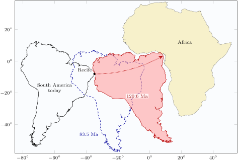
The fit of the coasts of South America and Africa, long noticed on maps, becomes a calculation. With the rotation of $120.6\,\mathrm{Ma}$, the coast of north-east Brazil near Recife ($8.05{}^{\circ}$ S, $34.9{}^{\circ}$ W) lands at $3.4{}^{\circ}$ N, $8.3{}^{\circ}$ E, on the coast of the Gulf of Guinea, after a journey of about $5000\,\mathrm{km}$ along its small circle: an average opening of some $40\,\mathrm{mm}\,\mathrm{yr}^{-1}$. The fit is not perfect everywhere: for some fourteen million years before the ocean opened, the two continents were slowly stretched apart, and a tight reconstruction must first restore the stretched margins and rift basins on both sides.

History — Tectonics on a sphere

In 1965 Edward Bullard and two colleagues fitted the continents around the Atlantic by computer, with a least-squares criterion: the best fit follows the steep part of the continental edge, at a depth of 500 fathoms (about $900\,\mathrm{m}$), not the coastline. The same year Tuzo Wilson described a new class of faults, the transform faults, and their bearing on continental drift. In 1967 Dan McKenzie and Robert Parker showed, with the North Pacific as their example, that the aseismic areas of the surface move as rigid plates on a sphere. In 1968 Jason Morgan described the surface as crustal blocks bounded by rises, trenches and great faults, and Xavier Le Pichon tied sea-floor spreading to continental drift. Within three years, the drift of continents had become the kinematics of rigid caps on a sphere.

12.5 Measuring plate motions

The magnetic record of the ocean floor

Lava erupted at a ridge acquires, as it cools, a magnetization in the direction of the Earth’s field at that moment, and keeps it as it moves away from the ridge. Since the field reverses at irregular intervals, the ocean floor is magnetized in alternating directions, in bands parallel to the ridge.

Definition 12.14 (Marine magnetic anomaly; polarity chron; polarity timescale)

A marine magnetic anomaly is the difference between the intensity of the magnetic field measured at sea and the intensity of a reference model of the Earth’s main field at the same place: it is positive above crust magnetized in the direction of the present field, and negative above crust magnetized in the opposite direction. A polarity chron is an interval of time during which the field kept one polarity, named by a number and the letter n (normal, as today) or r (reversed). The geomagnetic polarity timescale is the sequence of polarity chrons with the ages of their boundaries.

The timescale is built by dating reversal sequences on land and in deep-sea sediment cores, and by matching the pattern of the ocean-floor anomalies, whose widths keep the relative durations of the chrons. The present normal chron, C1n, began $0.781\,\mathrm{Ma}$, and the field has reversed at irregular intervals: the timescale counts twenty-five normal intervals in the last eleven million years, some lasting more than a million years, others little more than ten thousand. The figure below shows that history, down to the end of chron C5n, and the stripes it writes on the floor of a slow and of a fast ridge.

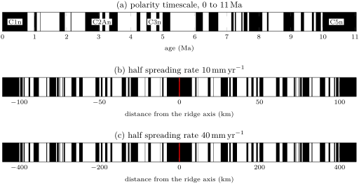
Definition 12.15 (Half and full spreading rates)

At a ridge, the half spreading rate of a flank is the rate at which the crust of that flank moves away from the ridge axis. The full spreading rate is the rate at which the two plates move apart, the sum of the two half rates; it is twice the half rate when the spreading is symmetric.

Method 12.16 (A spreading rate from magnetic anomalies)

1. On a magnetic profile perpendicular to the ridge, identify the sequence of anomalies on both flanks by its pattern of wide and narrow stripes, and match it to the polarity timescale.
2. Measure the distance from the axis to the same chron boundary on each flank, and divide by its age: these are the two half spreading rates, averaged since that time. The full rate is their sum, or the distance between the two boundaries divided by the age.
3. Prefer an old boundary to a young one: an error of a kilometre in a distance weighs less on a distance of a hundred kilometres than on one of ten.
4. If the profile is not perpendicular to the ridge, project the distances onto the direction of spreading.

The third point is not only a matter of reading errors. The crust does not acquire its magnetization along a single line: lava flows over the adjacent, slightly older crust, dykes intrude into it, and the lower crust is magnetized later than the upper. All these processes shift the boundaries between stripes away from the axis, so that the distance between two boundaries of the same age exceeds the width of crust actually formed. The two-sided shift is $1\text{ to }3\,\mathrm{km}$ at most ridges and reaches $5.0\,\mathrm{km}$ on the Reykjanes Ridge. Careful compilations correct the rates downward for this outward displacement, by $0.6\text{ to }2.6\,\mathrm{mm}\,\mathrm{yr}^{-1}$, and average them over the last $3.16\,\mathrm{Myr}$ on the slow ridges, back to the anomalies of chron C2An, and over $0.78\,\mathrm{Myr}$ on fast ones. On the Gakkel Ridge, starved of magma, the anomalies of the short Jaramillo subchron and of chron C2n are absent, while on the Reykjanes Ridge south of Iceland, spreading at less than $20\,\mathrm{mm}\,\mathrm{yr}^{-1}$ but with an abundant supply of magma, they are clearly recognized.

Satellite geodesy

Since the 1990s, the positions of permanent stations have been measured every day by satellite positioning. A series of daily positions over ten years or more gives a station’s velocity, once the seasonal movements and the jumps caused by earthquakes or by changes of equipment are dealt with (Exercise 12.12).

In the field — A permanent station

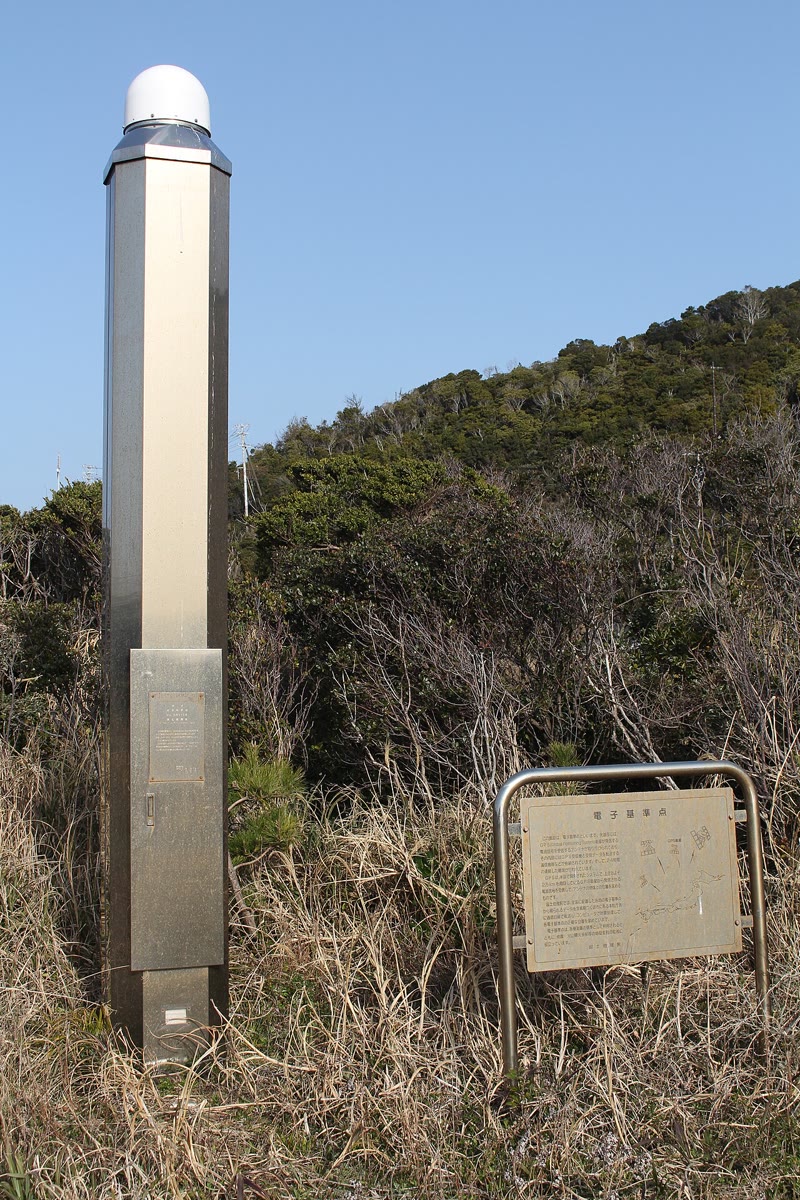
A permanent satellite-positioning station is a quiet instrument. The antenna, under its weatherproof dome, sits on top of a pillar or a braced mast cemented into rock, so that it moves with the crust and nothing else; the receiver in the base records the signals of every satellite in view, continuously, and sends them to a data centre. There, analysts compute a position for every day, in a reference frame tied to a worldwide network of stations, and publish time series and velocities. A station’s history matters as much as its data: each change of antenna or receiver is logged, because it can shift the computed position.

The velocities of stations in the interiors of two plates give an Euler vector of their own, independent of the geological record. For Eurasia relative to North America, such a vector predicts $17.0\,\mathrm{mm}\,\mathrm{yr}^{-1}$ in Iceland, about $8\,\%$ less than the $18.6\,\mathrm{mm}\,\mathrm{yr}^{-1}$ averaged over $3.16\,\mathrm{Myr}$ (figure above). The chord between Reykjavik and Stavanger, both on stable parts of their plates, lengthens by $17.5\,\mathrm{mm}\,\mathrm{yr}^{-1}$; the satellite vector predicts $17.1\,\mathrm{mm}\,\mathrm{yr}^{-1}$, the geological one $18.6\,\mathrm{mm}\,\mathrm{yr}^{-1}$. Across the North Atlantic, a rate measured over a few decades and a rate averaged over three million years thus agree to within a tenth: there, the plates move today nearly as they have moved for millions of years.

Inside the boundary zone the picture is less simple, for the stations move with more than the plates. More than a tenth of Iceland lies under ice caps, and most of them have been losing mass since about 1890: the crust beneath rises as the load decreases, and moves horizontally away from the thinning ice. The station at Höfn, on the south-east coast near the largest ice cap, rises by $12.9\,\mathrm{mm}\,\mathrm{yr}^{-1}$.

12.6 Exercises

Take $R = 6371\,\mathrm{km}$ throughout.

Exercise 12.1 ★

The Euler vector of Eurasia relative to North America has the rate $0.210{}^{\circ}/\mathrm{Myr}$. (a) Convert it to $\mathrm{rad}\,\mathrm{yr}^{-1}$ and to $\mathrm{rad}\,\mathrm{s}^{-1}$. (b) How long would a full turn take? (c) Compute $\omega R$ in $\mathrm{mm}\,\mathrm{yr}^{-1}$.

Solution

Solution of Exercise 12.1.

(a) $0.210{}^{\circ}/\mathrm{Myr} = 0.210\times\pi/180 = 3.665 \times 10^{-3}\,\mathrm{rad}$ per million years, that is $3.665 \times 10^{-9}\,\mathrm{rad}\,\mathrm{yr}^{-1}$; with $1\,\mathrm{yr} = 3.156 \times 10^{7}\,\mathrm{s}$, $1.161 \times 10^{-16}\,\mathrm{rad}\,\mathrm{s}^{-1}$. (b) $360/0.210 = 1714\,\mathrm{Myr}$, more than a third of the age of the Earth. (c) $\omega R = 3.665 \times 10^{-9}\times6.371 \times 10^{9}\,\mathrm{mm} = 23.35\,\mathrm{mm}\,\mathrm{yr}^{-1}$.

Exercise 12.2 ★

With the same Euler vector, compute the relative speed of the two plates at $30{}^{\circ}$, $60{}^{\circ}$ and $90{}^{\circ}$ from the Euler pole. Where along the plate boundary would the spreading be fastest?

Solution

Solution of Exercise 12.2.

$v = \omega R\sin\Delta = 23.35\sin\Delta$: $11.7\,\mathrm{mm}\,\mathrm{yr}^{-1}$ at $30{}^{\circ}$, $20.2\,\mathrm{mm}\,\mathrm{yr}^{-1}$ at $60{}^{\circ}$ and $23.35\,\mathrm{mm}\,\mathrm{yr}^{-1}$ at $90{}^{\circ}$. The spreading is fastest where the boundary is farthest from the pole, up to $90{}^{\circ}$: between Eurasia and North America, at the southern end of the boundary, near the Azores, $78{}^{\circ}$ from the pole.

Exercise 12.3 ★

The Jaramillo normal subchron lasted from $1.072\,\mathrm{Ma}$ to $0.988\,\mathrm{Ma}$. (a) How wide is the stripe it makes on each flank of a ridge with a half spreading rate of $50\,\mathrm{mm}\,\mathrm{yr}^{-1}$? Of $10\,\mathrm{mm}\,\mathrm{yr}^{-1}$? (b) What is the total width of the stripe of the present normal chron, which began $0.781\,\mathrm{Ma}$, on a ridge with a half rate of $10\,\mathrm{mm}\,\mathrm{yr}^{-1}$?

Solution

Solution of Exercise 12.3.

The subchron lasted $1.072 - 0.988 = 0.084\,\mathrm{Myr}$, and a half rate in $\mathrm{mm}\,\mathrm{yr}^{-1}$ is also a rate in $\mathrm{km}/\mathrm{Myr}$. (a) $50\times0.084 = 4.2\,\mathrm{km}$ at $50\,\mathrm{mm}\,\mathrm{yr}^{-1}$; $10\times0.084 = 0.84\,\mathrm{km}$ at $10\,\mathrm{mm}\,\mathrm{yr}^{-1}$. (b) The stripe straddles the axis: $2\times10\times0.781 = 15.6\,\mathrm{km}$.

Exercise 12.4 ★

On a profile across a ridge, the young edge of the anomaly of chron C2An, $2.581\,\mathrm{Ma}$ old, lies $66\,\mathrm{km}$ west of the axis and $64\,\mathrm{km}$ east of it. Compute the two half spreading rates and the full spreading rate. Is the spreading symmetric?

Solution

Solution of Exercise 12.4.

The half rates are $66/2.581 = 25.6\,\mathrm{mm}\,\mathrm{yr}^{-1}$ to the west and $64/2.581 = 24.8\,\mathrm{mm}\,\mathrm{yr}^{-1}$ to the east; the full rate is $130/2.581 = 50.4\,\mathrm{mm}\,\mathrm{yr}^{-1}$. The spreading is nearly symmetric: the western flank has grown about $3\,\%$ faster.

Exercise 12.5 ★★

A point of the Gakkel Ridge, in the Arctic Ocean, lies at $85{}^{\circ}$ N, $0{}^{\circ}$ E. Compute its angular distance from the Eurasia–North America Euler pole ($61.8{}^{\circ}$ N, $139.6{}^{\circ}$ E, $0.210{}^{\circ}/\mathrm{Myr}$) and the spreading rate there. Compare with the measured rates of $11\text{ to }12\,\mathrm{mm}\,\mathrm{yr}^{-1}$.

Solution

Solution of Exercise 12.5.

$\cos\Delta = \sin61.8{}^{\circ}\sin85{}^{\circ} + \cos61.8{}^{\circ}\cos85{}^{\circ} \cos(0{}^{\circ} - 139.6{}^{\circ}) = 0.8813\times0.9962 + 0.4726\times0.08716\times (-0.7615) = 0.87795 - 0.03137 = 0.84658$, so $\Delta = 32.16{}^{\circ}$ and $v = 23.35\sin32.16{}^{\circ} = 12.4\,\mathrm{mm}\,\mathrm{yr}^{-1}$. This is a little above the measured $11\text{ to }12\,\mathrm{mm}\,\mathrm{yr}^{-1}$, but the Euler vector is a single best fit to 453 rates, from which the rates depart by $0.7\,\mathrm{mm}\,\mathrm{yr}^{-1}$ on average, and individual rates near the slow Gakkel Ridge are among the least precise.

Exercise 12.6 ★★

At the Azores triple junction, $39.44{}^{\circ}$ N, $29.83{}^{\circ}$ W, compute (a) the angular distance to the Eurasia–North America Euler pole, (b) the spreading rate, and (c) the azimuth of the relative motion. (d) What trend do you predict for the transform faults of the ridge just north of the junction?

Solution

Solution of Exercise 12.6.

(a) $\cos\Delta = \sin61.8{}^{\circ}\sin39.44{}^{\circ} + \cos61.8{}^{\circ}\cos39.44{}^{\circ} \cos(169.43{}^{\circ}) = 0.20111$: $\Delta = 78.40{}^{\circ}$. (b) $v = 23.35 \sin78.40{}^{\circ} = 22.87\,\mathrm{mm}\,\mathrm{yr}^{-1}$, the $23\,\mathrm{mm}\,\mathrm{yr}^{-1}$ measured just north of the junction. (c) With the formula of the method, the numerator is $\sin169.43{}^{\circ}\cos61.8{}^{\circ} = 0.08668$ and the denominator $\cos39.44{}^{\circ}\sin61.8{}^{\circ} - \sin39.44{}^{\circ}\cos61.8{}^{\circ}\cos169.43{}^{\circ} = 0.97573$: the pole is seen at $\beta = 5.08{}^{\circ}$, nearly due north, and Eurasia moves towards $95.1{}^{\circ}$. (d) The transforms are parallel to the relative motion: they trend about $095{}^{\circ}$, nearly east–west.

Exercise 12.7 ★★

(a) Write the Euler vectors $\vec\omega_{\mathrm{EU\,NA}}$ ($61.8{}^{\circ}$ N, $139.6{}^{\circ}$ E, $0.210{}^{\circ}/\mathrm{Myr}$) and $\vec\omega_{\mathrm{NB\,NA}}$ ($79.2{}^{\circ}$ N, $40.2{}^{\circ}$ E, $0.233{}^{\circ}/\mathrm{Myr}$) in Cartesian components, in ${}^{\circ}/\mathrm{Myr}$. (b) Deduce $\vec\omega_{\mathrm{NB\,EU}}$, its pole and its rate. (c) Why is this the best way to know the motion of Nubia relative to Eurasia?

Solution

Solution of Exercise 12.7.

(a) $\vec\omega = \omega(\cos\varphi_p\cos\lambda_p, \cos\varphi_p\sin\lambda_p, \sin\varphi_p)$: $\vec\omega_{\mathrm{EU\,NA}} = (-0.0756, 0.0643, 0.1851)$ and $\vec\omega_{\mathrm{NB\,NA}} = (0.0333, 0.0282, 0.2289)$, in ${}^{\circ}/\mathrm{Myr}$. (b) $\vec\omega_{\mathrm{NB\,EU}} = \vec\omega_{\mathrm{NB\,NA}} - \vec\omega_{\mathrm{EU\,NA}} = (0.1089, -0.0361, 0.0438)$, of length

$$\sqrt{0.011859 + 0.001303 + 0.001918} = 0.1228{}^{\circ}/\mathrm{Myr}.$$

Its pole is at latitude $\arcsin(0.0438/0.1228) = 20.9{}^{\circ}$ N and longitude $\arctan(-0.0361/0.1089) = -18.3{}^{\circ}$, that is $18.3{}^{\circ}$ W (the $x$ component being positive, no $180{}^{\circ}$ is added). (c) The boundary between Nubia and Eurasia offers few direct measurements: between the Azores and Gibraltar, only the azimuths of the Gloria fault. The two spreading motions across the Atlantic are measured by hundreds of rates, and their difference inherits their precision.

Exercise 12.8 ★★

Let $\vec e_x$ point to $0{}^{\circ}$ N, $0{}^{\circ}$ E, $\vec e_y$ to $0{}^{\circ}$ N, $90{}^{\circ}$ E and $\vec e_z$ to the north pole. With Rodrigues’ formula, compute the image of $\vec e_x$ (a) by the rotation of $90{}^{\circ}$ about $\vec e_z$ followed by the rotation of $90{}^{\circ}$ about $\vec e_x$; (b) by the same two rotations in the opposite order. (c) What does this mean for the reconstruction of a plate’s past positions?

Solution

Solution of Exercise 12.8.

(a) About $\vec e_z$ by $90{}^{\circ}$: $\cos90{}^{\circ} = 0$, $\vec e_z\cdot\vec e_x = 0$ and $\vec e_z\times\vec e_x = \vec e_y$, so $\vec e_x$ goes to $\vec e_y$. Then about $\vec e_x$ by $90{}^{\circ}$: $\vec e_x\cdot\vec e_y = 0$ and $\vec e_x\times\vec e_y = \vec e_z$, so $\vec e_y$ goes to $\vec e_z$: the point ends at the north pole. (b) About $\vec e_x$ first: $\vec e_x$ is on the axis, $\vec e_x\times\vec e_x = \vec 0$ and $(1 - \cos90{}^{\circ})(\vec e_x\cdot\vec e_x) \vec e_x = \vec e_x$, so it does not move; then about $\vec e_z$ it goes to $\vec e_y$, at $0{}^{\circ}$ N, $90{}^{\circ}$ E. (c) The results differ: finite rotations do not commute. Successive reconstructions must be composed by multiplying the rotation matrices in the right order, never by adding angles or poles.

Exercise 12.9 ★★

Three plates A, B and C meet at a ridge–ridge–ridge junction. Relative to A, plate B moves at $30\,\mathrm{mm}\,\mathrm{yr}^{-1}$ towards the east and plate C at $40\,\mathrm{mm}\,\mathrm{yr}^{-1}$ towards the south. (a) Draw the velocity triangle. (b) Compute the speed and azimuth of C relative to B. (c) What is the trend of the ridge between B and C if it spreads perpendicular to its axis?

Solution

Solution of Exercise 12.9.

(a) In velocity space put $a$ at the origin, $b$ $30\,\mathrm{mm}\,\mathrm{yr}^{-1}$ to the east and $c$ $40\,\mathrm{mm}\,\mathrm{yr}^{-1}$ to the south. (b) $\vec v_{CB} = \vec v_{CA} - \vec v_{BA} = (0, -40) - (30, 0) = (-30, -40)$ (east, north components): $50\,\mathrm{mm}\,\mathrm{yr}^{-1}$ towards the azimuth $\arctan\bigl((-30)/(-40)\bigr) + 180{}^{\circ} = 216.9{}^{\circ}$, south-west. (c) The ridge is perpendicular to this direction: it trends $216.9{}^{\circ} - 90{}^{\circ} = 126.9{}^{\circ}$, that is north-west–south-east.

Exercise 12.10 ★★★

(a) Show that the trace of the matrix $R$ of a rotation by $\alpha$ about any axis is $1 + 2\cos\alpha$. (b) The matrix

$$R = \begin{pmatrix} 0 & 0 & 1\\ 1 & 0 & 0\\ 0 & 1 & 0\end{pmatrix}$$

is orthogonal with determinant $1$. Find its axis, as a latitude and longitude, and its angle. (c) Check your answer by applying $R$ to $\vec e_x$, $\vec e_y$ and $\vec e_z$.

Solution

Solution of Exercise 12.10.

(a) In Rodrigues’ matrix, the identity contributes $3\cos\alpha$, the matrix $\vec n\,\vec n^{\mathsf T}$ the trace $n_x^2 + n_y^2 + n_z^2 = 1$, times $1 - \cos\alpha$, and the antisymmetric matrix nothing: $\operatorname{tr}R = 3\cos\alpha + 1 - \cos\alpha = 1 + 2\cos\alpha$. (b) Here $\operatorname{tr}R = 0$, so $\cos\alpha = -1/2$ and $\alpha = 120{}^{\circ}$. The axis satisfies $R\vec n = \vec n$: $R(x, y, z) = (z, x, y)$, so $x = y = z$ and $\vec n = (1, 1, 1)/\sqrt3$, at latitude $\arcsin(1/\sqrt3) = 35.26{}^{\circ}$ N and longitude $45{}^{\circ}$ E. (c) $R\vec e_x = \vec e_y$, $R\vec e_y = \vec e_z$, $R\vec e_z = \vec e_x$: the three axes are permuted, as a third of a turn about the diagonal does. Rodrigues’ formula with $\alpha = +120{}^{\circ}$ about $\vec n$ indeed gives $\vec e_x\mapsto -\tfrac12\vec e_x + \tfrac12(1, 1, 1) + \tfrac{\sqrt3}{2}\cdot\tfrac{1}{\sqrt3}(0, 1, -1) = (0, 1, 0)$, so the rotation is anticlockwise seen from above $35.26{}^{\circ}$ N, $45{}^{\circ}$ E.

Exercise 12.11 ★★★

Before satellite positioning, Euler poles were found from the trends of transform faults. (a) Show that the Euler pole lies on the great circle through a point of a transform fault that is perpendicular to the fault there, and that the pole is therefore along $\vec t_1\times\vec t_2$, where $\vec t_1$ and $\vec t_2$ are unit vectors along two transform faults of the same boundary. (b) Transform faults trend at $95{}^{\circ}$ near the Azores triple junction ($39.44{}^{\circ}$ N, $29.83{}^{\circ}$ W) and at $103{}^{\circ}$ in Iceland ($64.5{}^{\circ}$ N, $18{}^{\circ}$ W). The horizontal unit vector at latitude $\varphi$ and longitude $\lambda$ pointing towards the azimuth $\beta$ is $\sin\beta\,\vec e + \cos\beta\,\vec n$, with $\vec e = (-\sin\lambda, \cos\lambda, 0)$ and $\vec n = (-\sin\varphi\cos\lambda, -\sin\varphi\sin\lambda, \cos\varphi)$. Locate the pole. (c) How well do two transforms determine the pole?

Solution

Solution of Exercise 12.11.

(a) On a transform the relative velocity $\vec\omega\times\vec r$ is along the fault, so parallel to $\vec t$; it is perpendicular to $\vec\omega$, hence $\vec t\cdot\vec\omega = 0$. The plane perpendicular to $\vec t$ through the centre contains $\vec r$ (since $\vec t$ is horizontal) and $\vec\omega$: it is the plane of the great circle through the point perpendicular to the fault, and the pole lies on that circle. Two such planes meet along the line of $\vec t_1\times\vec t_2$. (b) $\vec t_1 = (0.5436, 0.8367, -0.0673)$ at the junction and $\vec t_2 = (0.4942, 0.8639, -0.0968)$ in Iceland, so $\vec t_1\times\vec t_2 = (-0.02285, 0.01936, 0.05612)$, of length $0.06362$. Its latitude is $\arcsin(0.05612/0.06362) = 61.9{}^{\circ}$ N and its longitude $180{}^{\circ} - \arctan(0.01936/0.02285) = 139.7{}^{\circ}$ E (negative $x$ component): the pole of the chapter. (c) Badly: the two great circles cross at a small angle, since the trends differ by only $8{}^{\circ}$ over $26{}^{\circ}$ of the boundary. Changing either trend by one degree moves the pole by about $15{}^{\circ}$. Real determinations combine many transforms with spreading rates, whose variation along the boundary fixes the angular distance to the pole.

Exercise 12.12 ★★★

The eastward position of a station, every three months for three years, is (in millimetres, from $t = 0$):

$t$ (yr)	0	0.25	0.5	0.75	1	1.25	1.5	1.75	2	2.25	2.5	2.75	3
$x$ (mm)	4	5	6	15	24	25	26	65	74	75	76	85	94

It is made of a steady motion, a seasonal oscillation and a jump caused by an earthquake. (a) Compute the velocity from the first and last positions. (b) Compute the nine differences between positions exactly one year apart, and their median. (c) Explain why the median of one-year differences is a robust estimate of the steady velocity, and when it would fail.

Solution

Solution of Exercise 12.12.

(a) $(94 - 4)/3 = 30\,\mathrm{mm}\,\mathrm{yr}^{-1}$. (b) The differences one year apart are $24 - 4 = 20$, $25 - 5 = 20$, $26 - 6 = 20$, $65 - 15 = 50$, $74 - 24 = 50$, $75 - 25 = 50$, $76 - 26 = 50$, $85 - 65 = 20$ and $94 - 74 = 20$ (mm). Sorted: five values of 20 and four of 50; the median is $20\,\mathrm{mm}\,\mathrm{yr}^{-1}$. (c) Two positions one year apart are at the same phase of the seasonal oscillation, which cancels in their difference. A jump affects only the pairs that straddle it, here four of the nine; as long as fewer than half the pairs straddle a jump, the median ignores it, while the end-point estimate in (a) takes the whole jump as motion and comes out $50\,\%$ too high. The method fails when jumps are so frequent that most one-year pairs contain one, or when the station moves unsteadily, for instance after a large earthquake.

12.7 Problem: Iceland splits

Problem 12.1

Weekend problem — the opening of the North Atlantic across Iceland, measured three ways

Iceland sits on the Mid-Atlantic Ridge, between the North American plate to the west and the Eurasian plate to the east. Take $R = 6371\,\mathrm{km}$ and, for Eurasia relative to North America, the Euler vector with its pole at $61.8{}^{\circ}$ N, $139.6{}^{\circ}$ E and the rate $0.210{}^{\circ}/\mathrm{Myr}$.

Part I — The plate vector.

1. Convert the rate to $\mathrm{rad}\,\mathrm{yr}^{-1}$ and compute $\omega R$ in $\mathrm{mm}\,\mathrm{yr}^{-1}$.
2. Compute the angular distance $\Delta$ from the pole to the centre of Iceland, $64.5{}^{\circ}$ N, $18{}^{\circ}$ W.
3. Deduce the full spreading rate across Iceland predicted by the plate vector.
4. Compute the azimuth of the pole seen from Iceland, and the azimuth of the motion of Eurasia relative to North America.
5. Resolve this velocity into its eastward and northward components.
6. On the Gakkel Ridge, at $86{}^{\circ}$ N, $60{}^{\circ}$ E, what rate does the same vector give? Why is the boundary there so much slower?

Part II — The magnetic stripes. A ship’s magnetic profile across the Reykjanes Ridge, south-west of Iceland near $63{}^{\circ}$ N, $23{}^{\circ}$ W, run in the direction of spreading, gives the following distances from the axis to three chron boundaries (a profile constructed for this problem):

boundary	age (Ma)	west of the axis (km)	east of the axis (km)
base of C1n	0.781	9.7	10.1
young edge of C2An	2.581	26.8	27.3
young edge of C5n	9.779	94	97

7. From the young edge of C5n, compute the two half spreading rates.
8. Deduce the full spreading rate since $9.8\,\mathrm{Ma}$.
9. Compute the full rate from the two younger boundaries as well. Do the three agree? Describe how they change with the age of the boundary.
10. Is the spreading symmetric? Does the asymmetry change the full rate?
11. On the Reykjanes Ridge, the boundaries between stripes are displaced away from the axis by $5.0\,\mathrm{km}$ in all, both flanks together. Correct the three full rates. Why did the correction matter most for the youngest boundary?
12. How wide is the stripe of the Jaramillo subchron ($1.072\text{ to }0.988\,\mathrm{Ma}$) on each flank, at the corrected half rate? Compare with the displacement of question 11. The Jaramillo anomaly is nevertheless clearly recognized on Reykjanes Ridge profiles, but is absent from the Gakkel Ridge: what does that suggest?
13. The plate vector predicts $19.0\,\mathrm{mm}\,\mathrm{yr}^{-1}$ at the profile. Compare with your corrected rates.

Part III — The satellites. The permanent stations REYK (Reykjavik, $64.139{}^{\circ}$ N, $21.955{}^{\circ}$ W) and STAS (Stavanger, $59.018{}^{\circ}$ N, $5.599{}^{\circ}$ E) lie on the North American and Eurasian plates. Their measured velocities make the chord between them lengthen by $17.5\,\mathrm{mm}\,\mathrm{yr}^{-1}$.

14. Compute the angular distance between the two stations, and the length of the chord.
15. How long does the chord take to lengthen by one metre?
16. The plate vector gives STAS a velocity of $18.9\,\mathrm{mm}\,\mathrm{yr}^{-1}$ towards $114.8{}^{\circ}$ relative to North America. The great circle from REYK arrives at STAS heading towards $123.1{}^{\circ}$. Compute the component of the velocity along this direction, then the predicted lengthening of the chord, which makes the angle $\Delta/2$ with the horizontal at STAS.
17. Compare the measured and the predicted lengthening. What might explain the difference?
18. Relative to North America, REYK moves at $1.07\,\mathrm{mm}\,\mathrm{yr}^{-1}$ to the west and $0.97\,\mathrm{mm}\,\mathrm{yr}^{-1}$ to the south, and the station HOFN (Höfn, south-east Iceland) at $21.12\,\mathrm{mm}\,\mathrm{yr}^{-1}$ to the east and $6.97\,\mathrm{mm}\,\mathrm{yr}^{-1}$ to the south. Compute the speed and azimuth of HOFN relative to REYK.
19. Compare with Part I. HOFN also rises by $12.9\,\mathrm{mm}\,\mathrm{yr}^{-1}$. Why are stations inside Iceland a poor measure of the plate motion?

Part IV — Ten million years, and the junction to the south.

20. Over $10\,\mathrm{Myr}$, through what angle does Eurasia turn relative to North America about the pole?
21. How far does a point of Eurasia in the middle of Iceland travel along its small circle in that time? Compare with the corrected width of the crust formed since the young edge of C5n in Part II.
22. At the Azores triple junction, the plate vectors give Eurasia $22.9\,\mathrm{mm}\,\mathrm{yr}^{-1}$ towards $95.1{}^{\circ}$ and Nubia $19.2\,\mathrm{mm}\,\mathrm{yr}^{-1}$ towards $103.8{}^{\circ}$, both relative to North America. Compute the velocity of Eurasia relative to Nubia.
23. Is this junction stable? What kind of boundary does the velocity of question 22 imply between Eurasia and Nubia?
24. Gather the opening rates of Parts I, II and III. Which agree, and which method measures the motion of the plates over the shortest time?
25. To the nearest millimetre a year, what full spreading rate across Iceland do the plate vector and the corrected magnetic stripes both give?

Solution

Solution of Problem 12.1.

1. $\omega = 0.210\times(\pi/180)/10^{6} = 3.665 \times 10^{-9}\,\mathrm{rad}\,\mathrm{yr}^{-1}$; $\omega R = 3.665 \times 10^{-9}\times6.371 \times 10^{9}\,\mathrm{mm} = 23.35\,\mathrm{mm}\,\mathrm{yr}^{-1}$.

2. $\cos\Delta = \sin61.8{}^{\circ}\sin64.5{}^{\circ} + \cos61.8{}^{\circ} \cos64.5{}^{\circ}\cos(-157.6{}^{\circ}) = 0.79546 - 0.18809 = 0.60737$, so $\Delta = 52.60{}^{\circ}$.

3. $v = 23.35\sin52.60{}^{\circ} = 23.35\times0.7944 = 18.55\,\mathrm{mm}\,\mathrm{yr}^{-1}$.

4. The numerator is $\sin157.6{}^{\circ}\cos61.8{}^{\circ} = 0.18011$ and the denominator

$$\cos64.5{}^{\circ}\sin61.8{}^{\circ} - \sin64.5{}^{\circ}\cos61.8{}^{\circ}\cos157.6{}^{\circ} = 0.37940 + 0.39436 = 0.77376;$$

both are positive, so $\beta = \arctan 0.2328 = 13.1{}^{\circ}$. Eurasia moves towards $13.1{}^{\circ} + 90{}^{\circ} = 103.1{}^{\circ}$.

5. East: $18.55\sin103.1{}^{\circ} = 18.07\,\mathrm{mm}\,\mathrm{yr}^{-1}$; north: $18.55\cos103.1{}^{\circ} = -4.20\,\mathrm{mm}\,\mathrm{yr}^{-1}$, that is $4.20\,\mathrm{mm}\,\mathrm{yr}^{-1}$ to the south.

6. $\cos\Delta = 0.8851$, $\Delta = 27.74{}^{\circ}$, $v = 23.35 \sin27.74{}^{\circ} = 10.9\,\mathrm{mm}\,\mathrm{yr}^{-1}$. The two plates turn about a pole in eastern Siberia: the Gakkel Ridge is close to it, and the speed falls with $\sin\Delta$ although the plates are the same.

7. West: $94/9.779 = 9.61\,\mathrm{mm}\,\mathrm{yr}^{-1}$; east: $97/9.779 = 9.92\,\mathrm{mm}\,\mathrm{yr}^{-1}$.

8. $(94 + 97)/9.779 = 191/9.779 = 19.53\,\mathrm{mm}\,\mathrm{yr}^{-1}$.

9. From C2An: $54.1/2.581 = 20.96\,\mathrm{mm}\,\mathrm{yr}^{-1}$; from the base of C1n: $19.8/0.781 = 25.35\,\mathrm{mm}\,\mathrm{yr}^{-1}$. They do not agree: the younger the boundary, the higher the rate. A real change of rate is possible, but a steady excess in the distances, the same at all ages, would do exactly this.

10. The ratio of the west to the east distances is 0.96 to 0.98: the eastern flank has grown a few per cent more. The full rate depends only on the sum of the two distances, so the asymmetry does not change it.

11. $(191 - 5.0)/9.779 = 19.02\,\mathrm{mm}\,\mathrm{yr}^{-1}$; $(54.1 - 5.0)/2.581 = 19.02\,\mathrm{mm}\,\mathrm{yr}^{-1}$; $(19.8 - 5.0)/0.781 = 18.95\,\mathrm{mm}\,\mathrm{yr}^{-1}$. The three now agree within $0.1\,\mathrm{mm}\,\mathrm{yr}^{-1}$. The same $5\,\mathrm{km}$ is a quarter of the $19.8\,\mathrm{km}$ of the youngest pair but less than $3\,\%$ of the $191\,\mathrm{km}$ of the oldest; old boundaries give the more reliable rates.

12. The corrected half rate is $186/9.779/2 = 9.51\,\mathrm{mm}\,\mathrm{yr}^{-1}$, and $9.51\times0.084 = 0.80\,\mathrm{km}$, a third of the $2.5\,\mathrm{km}$ by which each boundary is displaced. One would expect so narrow a stripe to be blurred away. That it is recognized on the Reykjanes Ridge, while it is absent on the Gakkel Ridge, which is starved of magma, suggests that an abundant supply of magma records the field faithfully even in narrow stripes.

13. The corrected rates, 18.95 to $19.02\,\mathrm{mm}\,\mathrm{yr}^{-1}$, agree with the $19.0\,\mathrm{mm}\,\mathrm{yr}^{-1}$ of the plate vector; without the correction they exceeded it by 3 to 33 per cent.

14. $\cos\Delta = \sin64.139{}^{\circ}\sin59.018{}^{\circ} + \cos64.139{}^{\circ}\cos59.018{}^{\circ}\cos27.554{}^{\circ} = 0.97054$, so $\Delta = 13.94{}^{\circ}$; the chord is $2R\sin(\Delta/2) = 12742\times\sin6.97{}^{\circ} = 1546\,\mathrm{km}$.

15. $1000/17.5 = 57$ years.

16. The two directions differ by $123.1{}^{\circ} - 114.8{}^{\circ} = 8.3{}^{\circ}$: the horizontal component along the great circle is $18.9\cos8.3{}^{\circ} = 18.70\,\mathrm{mm}\,\mathrm{yr}^{-1}$, and along the chord $18.70\cos6.97{}^{\circ} = 18.56\,\mathrm{mm}\,\mathrm{yr}^{-1}$, about $18.6\,\mathrm{mm}\,\mathrm{yr}^{-1}$.

17. The chord lengthens by $17.5\,\mathrm{mm}\,\mathrm{yr}^{-1}$, $6\,\%$ less than the $18.6\,\mathrm{mm}\,\mathrm{yr}^{-1}$ predicted. Both stations stand far from the plate boundary, so the difference is not local. Either the plates move slightly more slowly today than on average over the last three million years, or one of the two estimates carries a small systematic error; the measurements alone cannot tell. An Euler vector computed from satellite positioning alone predicts $17.1\,\mathrm{mm}\,\mathrm{yr}^{-1}$ for this chord, close to the measured value.

18. East: $21.12 - (-1.07) = 22.19\,\mathrm{mm}\,\mathrm{yr}^{-1}$; north: $-6.97 - (-0.97) = -6.00\,\mathrm{mm}\,\mathrm{yr}^{-1}$. Speed $\sqrt{22.19^2 + 6.00^2} = 23.0\,\mathrm{mm}\,\mathrm{yr}^{-1}$, towards $180{}^{\circ} - \arctan(22.19/6.00) = 105.1{}^{\circ}$.

19. The direction is close to the $103{}^{\circ}$ of the plate vector, but the speed exceeds its $18.6\,\mathrm{mm}\,\mathrm{yr}^{-1}$ by a quarter. Both stations stand inside the zone where the boundary deforms, and Höfn, near the largest ice cap, moves with the rebound of the crust as the ice thins: up by $12.9\,\mathrm{mm}\,\mathrm{yr}^{-1}$, and sideways, away from the ice. Stations inside the boundary zone measure the plate motion plus local deformation.

20. $0.210\times10 = 2.10{}^{\circ}$.

21. The point travels on a small circle of radius $R\sin\Delta$: $6371\times0.7944\times(2.10\times\pi/180) = 185.5\,\mathrm{km}$. The corrected width of crust formed since the young edge of C5n, $186\,\mathrm{km}$ in $9.8\,\mathrm{Myr}$, is nearly the same: the motion has been steady over ten million years.

22. Components (east, north): Eurasia $(22.9\sin95.1{}^{\circ}, 22.9\cos95.1{}^{\circ}) = (22.81, -2.04)$, Nubia $(19.2\sin103.8{}^{\circ}, 19.2\cos103.8{}^{\circ}) = (18.65, -4.58)$. Eurasia relative to Nubia: $(4.16, 2.54)$, that is $4.9\,\mathrm{mm}\,\mathrm{yr}^{-1}$ towards $\arctan(4.16/2.54) = 58.6{}^{\circ}$, east-north-east.

23. A junction of three ridges is stable whatever the velocities. The velocity of question 22 makes Eurasia and Nubia move apart, east-north-east to west-south-west: their boundary at the junction must open, slowly; it is the Terceira Rift, whose east-south-east trend makes the opening oblique.

24. Part I: $18.6\,\mathrm{mm}\,\mathrm{yr}^{-1}$ in the centre of Iceland ($19.0\,\mathrm{mm}\,\mathrm{yr}^{-1}$ at the profile of Part II). Part II: 18.95 to $19.02\,\mathrm{mm}\,\mathrm{yr}^{-1}$ once corrected. Part III: the Reykjavik–Stavanger chord lengthens by $17.5\,\mathrm{mm}\,\mathrm{yr}^{-1}$, where the plate vector predicts $18.6\,\mathrm{mm}\,\mathrm{yr}^{-1}$; the pair inside Iceland gives $23.0\,\mathrm{mm}\,\mathrm{yr}^{-1}$, which is not the plate motion. The plate vector and the stripes agree; the satellites differ by $6\,\%$. The stripes average over up to ten million years, the plate vector over $3.16\,\mathrm{Myr}$; the satellites measure the motion of the last twenty to thirty years.

25. The plate vector gives $18.55\,\mathrm{mm}\,\mathrm{yr}^{-1}$ across Iceland, and the corrected stripes $19.0\,\mathrm{mm}\,\mathrm{yr}^{-1}$ beside it: to the nearest millimetre a year, the full spreading rate across Iceland is $19\,\mathrm{mm}\,\mathrm{yr}^{-1}$.