9The Layered Earth

On 8 October 1909 an earthquake shook the Kupa valley, south-east of Zagreb.

Andrija Mohorovičić, who ran the observatory there, gathered the seismograms recorded across Europe and noticed something odd: up to a few hundred kilometres from the epicentre the first tremor came in one way, farther out a second kind of first arrival took over, as if part of the energy had found a faster road at depth. He explained it by a boundary some fifty kilometres down, below which the waves travel faster: the base of the crust. A century of such records, millions of them, has turned that first boundary into a reference model of the whole Earth, layer by layer, with its velocities, its density, its gravity and its pressure down to the centre. This chapter shows how a boundary is found from travel times, what the reference model says, how a density profile is drawn from seismic velocities alone and checked against the Earth’s mass and moment of inertia, which minerals make the mantle at each depth, what the core is made of, and where the rigid outer shell of the planet ends.

You already know

A P wave is a compression wave, an S wave a shear wave; S waves do not cross liquids, and the P and S shadow zones of the core give the radius of the liquid outer core (Book 2, grade 11). Waves are refracted at a boundary according to Snell’s law, $\sin i_1/v_1 = \sin i_2/v_2$ (physics). In a fluid at rest the pressure grows with depth as $\mathrm dP = \rho g\,\mathrm dz$ (physics, University Year 1). The crust, the mantle and the core were introduced in Book 1 (grade 6).

9.1 Seismic waves in a layered Earth

The speeds of seismic waves depend on the elastic moduli of the rock and on its density. The physics books derive them from the equations of continuum elasticity; here they are taken as known.

Proposition 9.1 (Seismic speeds)

In an isotropic elastic solid of density $\rho$, bulk modulus $K$ and shear modulus $\mu$, P and S waves travel at

$$v_P = \sqrt{\frac{K + \tfrac43\mu}{\rho}}, \qquad v_S = \sqrt{\frac{\mu}{\rho}}.$$

In a liquid $\mu = 0$: $v_S = 0$ and no S wave propagates.

Since $K$ and $\mu$ are positive, $v_P > v_S$ always: in PREM’s crust and mantle $v_P$ is about $1.8$ to $1.9$ times $v_S$, and P waves arrive first. Both speeds generally grow with depth, because pressure stiffens the rock more than it compresses it, so that rays bend back towards the surface; and at a few depths they jump.

Definition 9.2 (Seismic discontinuity, Moho, core–mantle and inner-core boundaries)

A seismic discontinuity is a surface inside the Earth across which the seismic speeds, the density or both change abruptly, over a thickness small compared with a seismic wavelength. The Mohorovičić discontinuity (or Moho) is the base of the crust, where $v_P$ jumps to about $8\,\mathrm{km}\,\mathrm{s}^{-1}$. The core–mantle boundary is the surface between the solid silicate mantle and the liquid outer core; the inner-core boundary is the surface between the liquid outer core and the solid inner core.

9.1.1 Refraction at a layer boundary

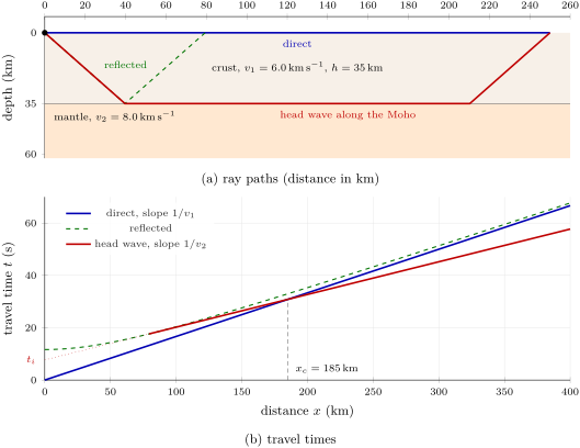
Take a layer of thickness $h$ and speed $v_1$, the crust, over a half-space of speed $v_2 > v_1$, the mantle, and a source at the surface. Three waves reach a receiver at the distance $x$. The direct wave travels in the layer, at $v_1$. The reflected wave bounces off the boundary. And a ray that strikes the boundary at the critical angle $i_c$, with $\sin i_c = v_1/v_2$, is refracted along it, travels in the faster medium just below it at the speed $v_2$, and sends energy back up into the layer at the same angle $i_c$ all along its way.

Definition 9.3 (Head wave, crossover distance)

A head wave is the wave that travels along a boundary at the speed of the faster medium below it and leaves it upward at the critical angle. The crossover distance is the distance from the source beyond which the head wave arrives before the direct wave.

Theorem 9.4 (Travel times over a two-layer Earth)

Over a layer of thickness $h$ and speed $v_1$ resting on a half-space of speed $v_2 > v_1$, a surface source and a surface receiver at the distance $x$ give

$$t_{\text{direct}} = \frac{x}{v_1}, \qquad t_{\text{head}} = \frac{x}{v_2} + \frac{2h\cos i_c}{v_1} \quad (x \ge 2h\tan i_c), \qquad \sin i_c = \frac{v_1}{v_2},$$

and the head wave arrives first beyond the crossover distance

$$x_c = 2h\sqrt{\frac{v_2 + v_1}{v_2 - v_1}}.$$

On a plot of travel time against distance, the direct and head waves are two straight lines. Their slopes are the inverse speeds $1/v_1$ and $1/v_2$; the head-wave line, extended back to $x = 0$, cuts the time axis at the intercept time $t_i = 2h\cos i_c/v_1$. The reflected wave, $t = \sqrt{x^2 + 4h^2}/v_1$, is a hyperbola that touches the head-wave line at the critical distance $2h\tan i_c$, where the head wave is born (Exercise 9.10).

Method 9.5 (The depth of a boundary from a refraction profile)

1. Plot the first-arrival times against distance, and fit one straight line through the arrivals close to the source and another through the distant ones.
2. The inverse slopes give $v_1$ and $v_2$; then $\sin i_c = v_1/v_2$.
3. Read the intercept time $t_i$ of the distant line at $x = 0$, and compute $h = t_i v_1/(2\cos i_c)$; check it with the crossover distance, $h = \tfrac12 x_c\sqrt{(v_2 - v_1)/(v_2 + v_1)}$.
4. A boundary is found only if $v_2 > v_1$: a slower layer below a faster one produces no head wave and stays hidden.

Mohorovičić’s two kinds of first arrival were exactly these two lines: the direct wave in the crust near the source, the head wave along the top of the mantle farther out. His figure for the thickness of the crust in that region, $54\,\mathrm{km}$, has been confirmed in its order of size, but the depth of the Moho varies from place to place. Under the oceans the crust is only about $5\,\mathrm{km}$ thick; under the continents it averages about $30\,\mathrm{km}$, and it is much thicker under large mountain ranges. For its reference model, PREM took the Moho at $11\,\mathrm{km}$ below sea level under the oceans and $35\,\mathrm{km}$ under the continents.

History — Andrija Mohorovičić

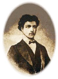
Andrija Mohorovičić (1857–1936) came to seismology from meteorology: a teacher, then from 1891 to 1921 the director of the meteorological observatory of Zagreb, he published his last meteorological study in 1901. On the seismograms of the Kupa valley earthquake of 8 October 1909 he found two distinct pairs of P and S phases: near the source one kind of first tremor arrived first, farther away another, which had travelled faster at depth. His reading of these two arrivals as a direct wave and a wave refracted below a boundary gave the boundary that now bears his name, and the first measure of the thickness of the crust.

9.2 A reference Earth model

The same reasoning, applied to millions of travel times at all distances and to the periods of the Earth’s free oscillations (the whole planet rings like a bell after a large earthquake), gives the speeds at every depth.

Definition 9.6 (Reference Earth model)

A reference Earth model is a spherically symmetric Earth, given as the seismic speeds $v_P(r)$, $v_S(r)$, the density $\rho(r)$ and, in the fullest models, the attenuation as functions of the radius $r$ alone, that fits the observed travel times, free-oscillation periods, the Earth’s mass and its moment of inertia. The most widely used is PREM, the Preliminary Reference Earth Model (1981).

PREM was fitted to the radius $6371\,\mathrm{km}$, the mass $5.974 \times 10^{24}\,\mathrm{kg}$ and the moment-of-inertia factor $0.3308$ of the Earth. It divides the planet into a few regions joined by discontinuities, and its profiles (figure below) show at once the main layers.

Definition 9.7 (Crust, mantle, outer core, inner core)

The crust is the outer silicate layer above the Moho. The mantle is the solid silicate shell between the Moho and the core–mantle boundary, at a depth of about $2891\,\mathrm{km}$. The outer core is the liquid metallic shell between the core–mantle boundary and the inner-core boundary, at about $5150\,\mathrm{km}$ depth. The inner core is the solid metallic sphere below it, of radius about $1220\,\mathrm{km}$.

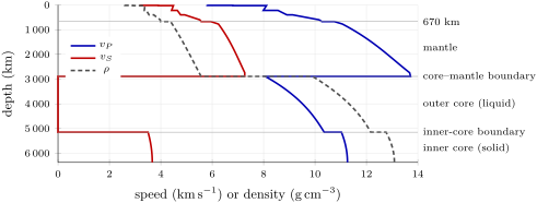
boundary in PREM	depth (km)	radius (km)	what changes
Moho	24.4	6346.6	crust above, peridotite below; $v_P$ 6.8 to 8.1
220-km discontinuity	220	6151	base of the low-velocity zone in PREM
400-km discontinuity	400	5971	olivine to wadsleyite ($410\,\mathrm{km}$ in most studies)
670-km discontinuity	670	5701	ringwoodite to bridgmanite and ferropericlase ($660\,\mathrm{km}$ in most studies)
core–mantle boundary	2891	3480	silicate to liquid iron; $v_S$ 7.3 to 0; $\rho$ 5.57 to 9.90
inner-core boundary	5149.5	1221.5	liquid to solid iron; $v_S$ 0 to 3.5; $\rho$ 12.17 to 12.76

Two facts in these profiles are directly observed. The vanishing of $v_S$ in the outer core is the S-wave shadow recalled above: S waves enter the core only as P waves, the core cannot transmit shear, so it is liquid. And the inner core transmits S waves, slowly: it is solid. That second fact came from weak P arrivals where no P wave should be.

History — Inge Lehmann and the inner core

Inge Lehmann (1888–1993), head of the seismological department of the Danish geodetic institute, studied the records of the 1929 Buller earthquake in New Zealand and found P waves arriving inside the shadow zone, where the core should have bent them away. In a paper of 1936 with the shortest of titles, P$'$, she showed that they could be explained if the core held a smaller inner core with a higher P speed, which returns part of the energy towards the surface. Her inner core is now known to be solid, and to grow slowly as the Earth cools. She also discovered the discontinuity near $220\,\mathrm{km}$ that bears her name.

9.3 Density, gravity and pressure from seismic data

Seismic speeds give two combinations of the moduli and the density, not the density itself. A third relation comes from the assumption that, inside a layer of uniform composition, the rock is simply compressed by the weight of the rock above.

Definition 9.8 (Seismic parameter)

The seismic parameter at a depth is

$$\Phi = v_P^2 - \tfrac43 v_S^2 = \frac{K}{\rho},$$

the bulk modulus divided by the density, computed from the two seismic speeds alone (Proposition 9.1).

Theorem 9.9 (Adams–Williamson equation)

In a region of uniform composition, in hydrostatic equilibrium, compressed adiabatically, the density varies with the radius as

$$\frac{\mathrm d\rho}{\mathrm dr} = -\frac{\rho(r)\,g(r)}{\Phi(r)},$$

where $g(r)$ is the gravity at the radius $r$.

The equation fails at a discontinuity, where the composition or the crystal structure changes, and wherever the temperature departs from the adiabat; but between the discontinuities it accounts for the observed increase of density with depth very well (panel (c) of the figure below). Starting from a density at the top of each region, integrating it downward, and adjusting the starting values until the mass and the moment of inertia come out right, is how the first density models were built. The two global numbers are integrals of the density.

Proposition 9.10 (Mass, gravity, pressure and moment of inertia)

For a spherically symmetric Earth of radius $R$ and density $\rho(r)$, the mass inside the radius $r$, the gravity, the pressure and the moment of inertia about an axis through the centre are

$$m(r) = \int_0^r 4\pi s^2\rho(s)\,\mathrm ds, \quad g(r) = \frac{G\,m(r)}{r^2}, \quad P(r) = \int_r^R \rho(s)\,g(s)\,\mathrm ds, \quad I = \frac{8\pi}{3}\int_0^R \rho(r)\,r^4\,\mathrm dr.$$

For a sphere of uniform density, $I = \tfrac{8\pi}{15}\rho R^5 = 0.4\,MR^2$. The Earth’s factor $I/MR^2 = 0.3308$ is smaller: its mass is concentrated towards the centre, which is the first argument for a dense core. Computed from PREM’s density alone, the integrals give a mass of $5.976 \times 10^{24}\,\mathrm{kg}$ ($0.06\,\%$ above the measured $5.972 \times 10^{24}\,\mathrm{kg}$), a factor $0.3309$, and a central pressure of $364\,\mathrm{GPa}$, the value tabulated with PREM to $0.1\,\%$.

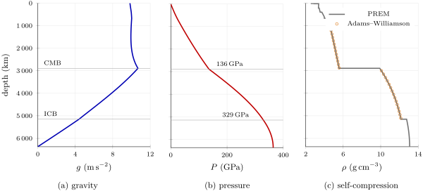
That gravity grows on the way down through the mantle is a direct consequence of the dense core: the mass left inside the radius falls more slowly than $r^2$. Through the mantle $g$ hardly changes, and the pressure grows almost linearly with depth, by about $4.7\,\mathrm{GPa}$ per hundred kilometres.

9.4 The mantle: one rock, several mineral assemblages

The upper mantle is peridotite, known from the fragments that volcanoes bring up and from slices of mantle thrust onto continents: about half to three fifths olivine by volume ($49\text{ to }62\,\%$ in the proposed compositions), the rest pyroxenes and an aluminous mineral (plagioclase, spinel or garnet, depending on depth). The pressure that rises with depth does not change this composition, but it forces its atoms into denser arrangements: polymorphs (Chapter 7) appear one after the other.

Definition 9.11 (Mantle transition zone)

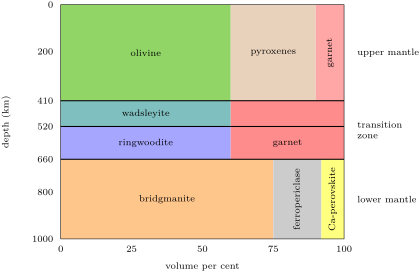
The mantle transition zone is the part of the mantle between the seismic discontinuities near $410\,\mathrm{km}$ and $660\,\mathrm{km}$ depth, in which olivine of the upper mantle is replaced by its denser polymorphs, wadsleyite and then ringwoodite. Above it is the upper mantle; below it the lower mantle, down to the core–mantle boundary.

At about $410\,\mathrm{km}$ ($14\,\mathrm{GPa}$) olivine $\ce{(Mg,Fe)2SiO4}$ becomes wadsleyite, of the same formula; near $520\,\mathrm{km}$ ($17.5\,\mathrm{GPa}$) wadsleyite becomes ringwoodite; the pyroxenes dissolve into a garnet rich in silicon, majorite, until by the middle of the transition zone garnet holds all of them, so that the zone is a little more than half olivine polymorphs and the rest garnet. At about $660\,\mathrm{km}$, at a pressure near $24\,\mathrm{GPa}$, ringwoodite breaks down into two minerals, written for the magnesian end-member

bridgmanite, $\ce{(Mg,Fe)SiO3}$ with the structure of perovskite, and ferropericlase, $\ce{(Mg,Fe)O}$. A lower mantle of the same composition as the upper mantle is about $75\,\%$ bridgmanite, $17\,\%$ ferropericlase and $8\,\%$ of a calcium silicate perovskite by volume, and fits the densities and speeds of the reference model. Bridgmanite is therefore the most abundant mineral of the Earth; it received its name only in 2014, after natural grains were described in a heavily shocked meteorite.

Each change produces denser minerals, so it raises the density and the seismic speeds: the transitions are the discontinuities of the profiles (figure below). Their depths are not fixed. A phase change happens at a pressure that depends on the temperature, and the slope of that dependence (the Clapeyron slope, treated in the next university volume) moves the $410\,\mathrm{km}$ discontinuity up and the $660\,\mathrm{km}$ down in the cold rock of a sinking slab. Mapping the topography of the discontinuities is one way of finding cold and hot regions in the mantle.

At the bottom of the mantle, the layer called D$''$ (D double prime, a name kept from an early model of the Earth) has a velocity gradient different from the rest of the lower mantle; PREM gives it the lowest $150\,\mathrm{km}$ of the mantle. It is seismically heterogeneous: patches of very low speed, steep gradients, reflectors. It is thought to be a boundary layer between the hot core and the mantle, and perhaps a graveyard of old slabs.

9.5 The core

The core is mostly iron. Its density, its speeds and its ability to generate a magnetic field all point to a metal, and iron is by far the most abundant element dense enough among those that the meteorites and the Sun show to be common. Nickel, abundant in iron meteorites, accompanies it. But the core is not pure iron–nickel.

• The core is $5\text{ to }10\,\%$ less dense than pure iron would be at the same pressure and temperature: it must contain light elements, among which silicon, sulfur, carbon, oxygen and hydrogen are the candidates.
• The density jumps by about $4.5\,\%$ at the inner-core boundary, too much for the freezing of one and the same metal: the inner core holds light elements too, but fewer, a few per cent against $5\text{ to }10\,\%$ in the liquid.

The difference has a consequence. As the Earth cools — its mantle by about $100{}^{\circ}\mathrm{C}$ per billion years at present — the liquid of the core freezes onto the inner core, which grows, and

freezing leaves most of the light elements in the liquid. The light liquid released at the bottom of the outer core rises, and this buoyancy is thought to help stir the outer core and drive the dynamo that makes the Earth’s magnetic field.

9.6 Mechanical layers: lithosphere and asthenosphere

The layers above are defined by composition and phase: crust and mantle are different rocks, outer and inner core different states. Plate tectonics needs a different division, by strength, which cuts across the first one.

Definition 9.12 (Lithosphere, asthenosphere, low-velocity zone)

The lithosphere is the rigid outer shell of the Earth, the crust and the uppermost mantle, which behaves as a strong layer over geological times and is divided into plates. The asthenosphere is the weaker layer of the upper mantle below it, which deforms by slow flow and lets the plates move. The low-velocity zone is the depth range below the lithosphere where the seismic speeds, S speeds especially, are lower than just above and below.

The lithosphere is not a rock but a temperature range: mantle peridotite is strong where it is cold and creeps where it is hot, and its base is roughly an isotherm. It is thin under ridges, where hot mantle rises, about $140\,\mathrm{km}$ thick under the oldest ocean floor, and $40\text{ to }280\,\mathrm{km}$ thick under continents, the thickest under old cratons; the top of the asthenosphere lies at about $80\text{ to }200\,\mathrm{km}$. Seismically, the asthenosphere shows as the low-velocity zone, close to its melting conditions: in PREM the S speed decreases slightly from the Moho down to $220\,\mathrm{km}$, where it jumps up again. How strength depends on temperature, and why it does so, is the subject of Chapter 16.

In the field — A seismic station

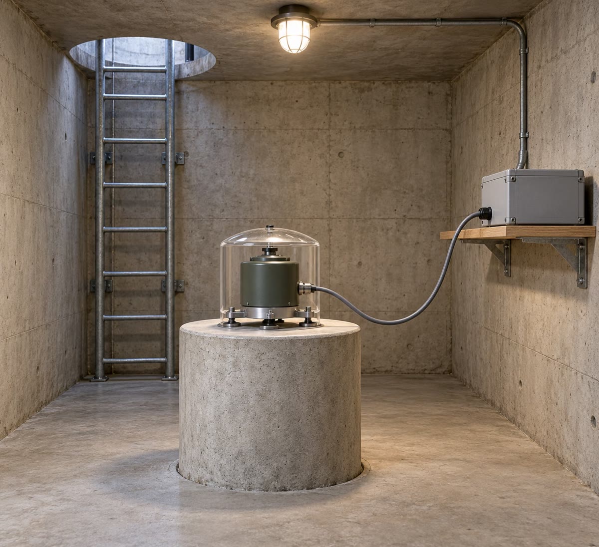
The travel times on which reference models rest come from permanent stations. A broadband seismometer, which records ground motions from hundredths of a second to hours in period, sits on a concrete pier set on bare rock and isolated from the floor of the vault, under a cover that keeps its temperature steady: a change of a fraction of a degree, a draught or a passing lorry would show on the record. The data logger stamps every sample with time from satellites, and the records stream to data centres that share them openly. Networks of such stations locate and time every large earthquake; arrival times picked on their records were inverted for the speeds at each depth.

9.7 Exercises

Exercise 9.1 ★

With the PREM radii $R = 6371\,\mathrm{km}$, $r_{\text{CMB}} = 3480\,\mathrm{km}$ and $r_{\text{ICB}} = 1221.5\,\mathrm{km}$, compute the fractions of the Earth’s volume occupied by the core and by the inner core.

Solution

Solution of Exercise 9.1.

The volume fractions are the cubes of the radius ratios: core $(3480/6371)^3 = 0.1630$, that is $16.3\,\%$; inner core $(1221.5/6371)^3 = 0.00705$, $0.70\,\%$.

Exercise 9.2 ★

Just above the core–mantle boundary PREM gives $v_P = 13.7166\,\mathrm{km}\,\mathrm{s}^{-1}$, $v_S = 7.264\,66\,\mathrm{km}\,\mathrm{s}^{-1}$, $\rho = 5.566\,45\,\mathrm{g}\,\mathrm{cm}^{-3}$; just below, $v_P = 8.064\,82\,\mathrm{km}\,\mathrm{s}^{-1}$, $v_S = 0$, $\rho = 9.903\,49\,\mathrm{g}\,\mathrm{cm}^{-3}$. Compute the seismic parameter and the bulk modulus on each side (in GPa). What changes most across the boundary?

Solution

Solution of Exercise 9.2.

Above: $\Phi = 13.7166^2 - \tfrac43\times7.26466^2 = 188.145 - 70.367 = 117.78\,\mathrm{km}^{2}\,\mathrm{s}^{-2}$, $K = \rho\Phi = 5566.45\,\mathrm{kg}\,\mathrm{m}^{-3}\times 117.78 \times 10^{6}\,\mathrm{m}^{2}\,\mathrm{s}^{-2} = 655.6\,\mathrm{GPa}$. Below: $\Phi = 8.06482^2 = 65.04\,\mathrm{km}^{2}\,\mathrm{s}^{-2}$, $K = 9903.49\times65.04 \times 10^{6} = 644.1\,\mathrm{GPa}$. The bulk modulus hardly changes ($-1.7\,\%$). What changes is the shear modulus, $\mu = \rho v_S^2 = 293.8\,\mathrm{GPa}$ above and $0$ below (a liquid), and the density, which rises by $78\,\%$: hence the drop of $v_P$ despite an almost equal $K$.

Exercise 9.3 ★

A crust $30\,\mathrm{km}$ thick, at $6.2\,\mathrm{km}\,\mathrm{s}^{-1}$, rests on a mantle at $8.1\,\mathrm{km}\,\mathrm{s}^{-1}$. Compute the critical angle, the critical distance and the crossover distance.

Solution

Solution of Exercise 9.3.

$\sin i_c = 6.2/8.1 = 0.7654$, $i_c = 49.95{}^{\circ}$. Critical distance $2\times30\times\tan49.95{}^{\circ} = 60\times1.1906 = 71.4\,\mathrm{km}$. Crossover distance $60\sqrt{14.3/1.9} = 60\times2.743 = 164.6\,\mathrm{km}$.

Exercise 9.4 ★

The core’s mass is $1.94 \times 10^{24}\,\mathrm{kg}$ and its radius $3480\,\mathrm{km}$. Compute the gravity at the core–mantle boundary and compare it with the surface gravity, $9.82\,\mathrm{m}\,\mathrm{s}^{-2}$. Why is it larger?

Solution

Solution of Exercise 9.4.

$g = Gm/r^2 = 6.674 \times 10^{-11}\times1.94 \times 10^{24}/(3.48 \times 10^{6})^2 = 10.69\,\mathrm{m}\,\mathrm{s}^{-2}$, $9\,\%$ more than at the surface. Going down to the core, the radius squared falls to $(3480/6371)^2 = 0.298$ of its surface value, while the attracting mass falls only to $1.94/5.972 = 0.325$ of the total, because the core holds a third of the mass: $0.325/0.298 = 1.09$.

Exercise 9.5 ★★

On a refraction profile the first arrivals are at $10.0\,\mathrm{s}$ at $60\,\mathrm{km}$, and at $33.3\,\mathrm{s}$ at $200\,\mathrm{km}$ and $45.8\,\mathrm{s}$ at $300\,\mathrm{km}$; the line through the first point passes through the origin. Find $v_1$, $v_2$, the intercept time and the depth of the boundary, and check the result with the crossover distance.

Solution

Solution of Exercise 9.5.

Near the source $v_1 = 60/10.0 = 6.0\,\mathrm{km}\,\mathrm{s}^{-1}$. Far away $v_2 = (300 - 200)/(45.8 - 33.3) = 100/12.5 = 8.0\,\mathrm{km}\,\mathrm{s}^{-1}$; the intercept time is $t_i = 33.3 - 200/8.0 = 8.3\,\mathrm{s}$. Then $\sin i_c = 0.75$, $\cos i_c = 0.6614$, and $h = t_i v_1/(2\cos i_c) = 8.3\times6.0/1.3229 = 37.6\,\mathrm{km}$. Check: $x_c = 2\times37.6\times\sqrt{14/2} = 199\,\mathrm{km}$, where both waves arrive at $199/6.0 = 199/8.0 + 8.3 = 33.2\,\mathrm{s}$.

Exercise 9.6 ★★

Show that a uniform sphere has $I = 0.4\,MR^2$. Then compute the mass and the factor $I/MR^2$ of a two-layer Earth: a core of radius $3480\,\mathrm{km}$ and density $11.0\,\mathrm{g}\,\mathrm{cm}^{-3}$ in a mantle of density $4.45\,\mathrm{g}\,\mathrm{cm}^{-3}$, with $R = 6371\,\mathrm{km}$. Compare with $5.972 \times 10^{24}$ kg and $0.3308$.

Solution

Solution of Exercise 9.6.

For uniform $\rho$, $I = \tfrac{8\pi}{3}\rho\int_0^R r^4\,\mathrm dr = \tfrac{8\pi}{15}\rho R^5$ and $M = \tfrac43\pi\rho R^3$, so $I/MR^2 = (8/15)/(4/3) = 0.4$. Two layers ($r_c = 3.48 \times 10^{6}\,\mathrm{m}$, $R = 6.371 \times 10^{6}\,\mathrm{m}$): $M = \tfrac43\pi\bigl(11000\,r_c^3 + 4450\,(R^3 - r_c^3)\bigr) = 5.977 \times 10^{24}\,\mathrm{kg}$, $0.08\,\%$ above the measured mass; $I = \tfrac{8\pi}{15}\bigl(11000\,r_c^5 + 4450\,(R^5 - r_c^5)\bigr)$ gives $I/MR^2 = 0.3457$. The mass is right, but the factor is $4.5\,\%$ too high: the real mantle is not uniform, its density grows with depth, which moves mass inward.

Exercise 9.7 ★★

At $1471\,\mathrm{km}$ depth PREM gives $v_P = 12.16\,\mathrm{km}\,\mathrm{s}^{-1}$, $v_S = 6.673\,\mathrm{km}\,\mathrm{s}^{-1}$, $\rho = 4.86\,\mathrm{g}\,\mathrm{cm}^{-3}$, and the gravity is $9.9\,\mathrm{m}\,\mathrm{s}^{-2}$. Compute the density gradient given by the Adams–Williamson equation, in $\mathrm{g}\,\mathrm{cm}^{-3}$ per $1000\,\mathrm{km}$, and compare with PREM’s densities, $4.844$ at $1471\,\mathrm{km}$ and $5.357$ at $2471\,\mathrm{km}$.

Solution

Solution of Exercise 9.7.

$\Phi = 12.16^2 - \tfrac43\times6.673^2 = 147.87 - 59.37 = 88.49\,\mathrm{km}^{2}\,\mathrm{s}^{-2}$. With depth $z$, $\mathrm d\rho/\mathrm dz = \rho g/\Phi = 4860\times9.9/88.49 \times 10^{6} = 5.44 \times 10^{-4}\,\mathrm{kg}\,\mathrm{m}^{-4}$, that is $0.544\,\mathrm{kg}\,\mathrm{m}^{-3}$ per kilometre, or $0.54\,\mathrm{g}\,\mathrm{cm}^{-3}$ per $1000\,\mathrm{km}$. PREM rises by $5.357 - 4.844 = 0.513$ over these $1000\,\mathrm{km}$, $6\,\%$ less: the gradient computed at the top is applied to the whole interval, while $\Phi$ grows with depth and the gradient decreases.

Exercise 9.8 ★★

Estimate the pressure at $670\,\mathrm{km}$ depth from a mean density of $3.57\,\mathrm{g}\,\mathrm{cm}^{-3}$ and a gravity of $9.9\,\mathrm{m}\,\mathrm{s}^{-2}$. Which mineral change is expected there?

Solution

Solution of Exercise 9.8.

$P \approx \bar\rho g z = 3570\times9.9\times670 \times 10^{3} = 23.7\,\mathrm{GPa}$ (PREM: $23.9\,\mathrm{GPa}$). It is the pressure, about $24\,\mathrm{GPa}$, at which ringwoodite breaks down into bridgmanite and ferropericlase: the $660\,\mathrm{km}$ discontinuity.

Exercise 9.9 ★★

PREM’s mean density of the outer core is $10.90\,\mathrm{g}\,\mathrm{cm}^{-3}$; at the inner-core boundary its density is $12.166\,\mathrm{g}\,\mathrm{cm}^{-3}$ above and $12.764\,\mathrm{g}\,\mathrm{cm}^{-3}$ below. (a) If iron at the same conditions is $5\text{ to }10\,\%$ denser than the outer core, what range of densities does that give for liquid iron there? (b) Compute the density jump at the inner-core boundary in per cent, and compare it with the $4.5\,\%$ of recent studies. (c) What does a jump larger than freezing alone would give say about the light elements?

Solution

Solution of Exercise 9.9.

(a) Liquid iron: $10.90\times1.05 = 11.4$ to $10.90\times1.10 = 12.0\,\mathrm{g}\,\mathrm{cm}^{-3}$. (b) $12.764/12.166 = 1.049$: a jump of $4.9\,\%$ in PREM, a little more than the $4.5\,\%$ of recent studies. (c) Freezing alone would make the solid only slightly denser than the liquid; the larger jump means that the solid holds fewer light elements than the liquid: they prefer the liquid, and freezing at the inner-core boundary leaves most of them behind.

Exercise 9.10 ★★★

Show that the reflected-wave time $t_r(x) = \sqrt{x^2 + 4h^2}/v_1$ and the head-wave time of Theorem 9.4 are equal, and have equal slopes, at $x = 2h\tan i_c$, and that $t_r > t_{\text{head}}$ beyond it. Interpret.

Solution

Solution of Exercise 9.10.

Let $x_* = 2h\tan i_c$. Then $\sqrt{x_*^2 + 4h^2} = 2h/\cos i_c$ and $t_r(x_*) = 2h/(v_1\cos i_c)$. The head wave gives $t(x_*) = 2h\tan i_c/v_2 + 2h\cos i_c/v_1 = \frac{2h}{v_1}\bigl(\sin^2 i_c/\cos i_c + \cos i_c\bigr) = 2h/(v_1\cos i_c)$, using $\sin i_c = v_1/v_2$: the same. The slope of the hyperbola is $t_r'(x) = x/(v_1\sqrt{x^2 + 4h^2})$; at $x_*$ it is $\sin i_c/v_1 = 1/v_2$, the slope of the head-wave line. Since $t_r'' > 0$, the hyperbola is convex and lies above each of its tangents: for $x > x_*$, $t_r > t_{\text{head}}$. At the critical distance the reflection strikes the boundary at exactly $i_c$ and is the head wave’s birth; beyond, the head wave, which gains by running in the fast medium, comes first.

Exercise 9.11 ★★★

For an Earth of uniform density $\rho$, show that $g(r) = \tfrac43\pi G\rho r$ and $P(r) = \tfrac23\pi G\rho^2(R^2 - r^2)$. Compute the central pressure with $\rho = 5513\,\mathrm{kg}\,\mathrm{m}^{-3}$ and $R = 6371\,\mathrm{km}$, and compare with PREM’s $363.85\,\mathrm{GPa}$.

Solution

Solution of Exercise 9.11.

$m(r) = \tfrac43\pi\rho r^3$, so $g = Gm/r^2 = \tfrac43\pi G\rho r$. Then $P(r) = \int_r^R \rho\,\tfrac43\pi G\rho s\,\mathrm ds = \tfrac23\pi G\rho^2(R^2 - r^2)$. At the centre $P = \tfrac23\pi\times6.674 \times 10^{-11}\times5513^2\times (6.371 \times 10^{6})^2 = 172\,\mathrm{GPa}$, $47\,\%$ of PREM’s $363.85\,\mathrm{GPa}$: concentrating the mass towards the centre roughly doubles the central pressure.

Exercise 9.12 ★★★

Show that if $g/\Phi$ is constant through a layer, the Adams–Williamson equation gives $\rho = \rho_0\exp\bigl(g(z - z_0)/\Phi\bigr)$ with depth $z$. Apply it to the outer core, from $2891\,\mathrm{km}$ ($\rho_0 = 9.90\,\mathrm{g}\,\mathrm{cm}^{-3}$) to $5149.5\,\mathrm{km}$, with mean values $g = 7.9\,\mathrm{m}\,\mathrm{s}^{-2}$ and $\Phi = 87\,\mathrm{km}^{2}\,\mathrm{s}^{-2}$; compare with PREM’s $12.17\,\mathrm{g}\,\mathrm{cm}^{-3}$ at the inner-core boundary.

Solution

Solution of Exercise 9.12.

With $z$ the depth, $\mathrm d\rho/\mathrm dz = \rho g/\Phi$; if $g/\Phi$ is a constant $a$, $\mathrm d(\ln\rho)/\mathrm dz = a$ and $\rho = \rho_0 e^{a(z - z_0)}$. Here $a(z - z_0) = 7.9\times2258.5 \times 10^{3}/87 \times 10^{6} = 0.2051$ and $\rho = 9.90\times e^{0.2051} = 9.90\times1.2276 = 12.15\,\mathrm{g}\,\mathrm{cm}^{-3}$, $0.2\,\%$ below PREM’s $12.17$: the whole increase of density through the outer core is self-compression.

9.8 Problem: Weighing the Earth’s shells

Problem 9.1

Weekend problem — volumes, masses and moment of inertia of a four-shell Earth built from PREM, compared with the measured mass and moment of inertia; gravity and pressure deep inside

The Earth is cut into four shells at the radii of PREM, and each is given its mean density in PREM, rounded:

shell	from (km)	to (km)	mean density ($\mathrm{g}\,\mathrm{cm}^{-3}$)
crust, upper mantle and transition zone	5701	6371	3.57
lower mantle	3480	5701	4.90
outer core	1221.5	3480	10.90
inner core	0	1221.5	12.89

Use $G = 6.674 \times 10^{-11}\,\mathrm{m}^{3}\,\mathrm{kg}^{-1}\,\mathrm{s}^{-2}$. The measured mass of the Earth is $5.972 \times 10^{24}\,\mathrm{kg}$ and its moment-of-inertia factor $I/MR^2 = 0.3308$.

Part I — Volumes.

1. Compute the volume of the Earth.
2. Compute the volume of each shell.
3. What fraction of the volume does each shell occupy? Which shell is the largest?
4. What fraction of the volume is core?

Part II — Masses.

5. Compute the mass of each shell.
6. Add them, and compare the total with the measured mass.
7. Deduce the mean density of the model Earth.
8. What fraction of the mass is in the inner core?
9. What fraction of the mass is in the mantle and crust together?
10. Compare the core’s share of the volume and of the mass, and explain.

Part III — Moment of inertia.

11. Show from Proposition 9.10 that a uniform shell between $r_1$ and $r_2$ has $I = \tfrac{8\pi}{15}\rho\,(r_2^5 - r_1^5)$.
12. Compute the moment of inertia of each shell.
13. Which shell contributes most, and why does the inner core contribute almost nothing?
14. Add them and compute $I/MR^2$ for the model.
15. Compare with $0.3308$ and with the $0.4$ of a uniform sphere.
16. Inside each real shell the density increases with depth. Does that explain why the model’s factor is too high? Explain.

Part IV — Gravity and pressure.

17. Compute the gravity at the surface of the model.
18. Compute the gravity at the core–mantle boundary.
19. Compute the mean density of the mantle and crust together.
20. Gravity in the mantle stays close to $10\,\mathrm{m}\,\mathrm{s}^{-2}$. Estimate the pressure at the core–mantle boundary, and compare with PREM’s $135.75\,\mathrm{GPa}$.
21. Compute the mean density of the core, and the pressure increase from the core–mantle boundary to the centre in a uniform core, $\tfrac23\pi G\rho_c^2 r_c^2$ (Exercise 9.11 applied to the core alone).
22. Add the two to estimate the central pressure, and compare with PREM’s $363.85\,\mathrm{GPa}$. Why is the estimate too low?
23. Which of the model’s numbers are checked against a measurement, and which only against PREM itself?
24. What fraction of the Earth’s mass lies in the core?

Solution

Solution of Problem 9.1.

1. $V = \tfrac43\pi(6.371 \times 10^{6})^3 = 1.0832 \times 10^{21}\,\mathrm{m}^{3}$.

2. $\tfrac43\pi(r_2^3 - r_1^3)$: crust, upper mantle and transition zone $3.0706 \times 10^{20}\,\mathrm{m}^{3}$; lower mantle $5.9961 \times 10^{20}\,\mathrm{m}^{3}$; outer core $1.6890 \times 10^{20}\,\mathrm{m}^{3}$; inner core $7.634 \times 10^{18}\,\mathrm{m}^{3}$.

3. $28.35\,\%$, $55.36\,\%$, $15.59\,\%$ and $0.70\,\%$: the lower mantle is the largest shell, more than half of the Earth’s volume.

4. $15.59 + 0.70 = 16.3\,\%$.

5. Crust, upper mantle and transition zone $3.0706 \times 10^{20}\times3570 = 1.0962 \times 10^{24}\,\mathrm{kg}$; lower mantle $2.9381 \times 10^{24}\,\mathrm{kg}$; outer core $1.8410 \times 10^{24}\,\mathrm{kg}$; inner core $9.841 \times 10^{22}\,\mathrm{kg}$.

6. $5.9737 \times 10^{24}\,\mathrm{kg}$, $0.03\,\%$ above the measured $5.972 \times 10^{24}\,\mathrm{kg}$.

7. $5.9737 \times 10^{24}/1.0832 \times 10^{21} = 5515\,\mathrm{kg}\,\mathrm{m}^{-3}$.

8. $9.841 \times 10^{22}/5.9737 \times 10^{24} = 1.65\,\%$.

9. $(1.0962 + 2.9381)/5.9737 = 67.5\,\%$.

10. The core is $16.3\,\%$ of the volume and $32.5\,\%$ of the mass, twice as much: its mean density, $10\,986\,\mathrm{kg}\,\mathrm{m}^{-3}$, is about $2.5$ times that of the mantle.

11. A shell of uniform density gives $I = \tfrac{8\pi}{3}\rho\int_{r_1}^{r_2} r^4\,\mathrm dr = \tfrac{8\pi}{15}\rho (r_2^5 - r_1^5)$.

12. Crust, upper mantle and transition zone $2.676 \times 10^{37}\,\mathrm{kg}\,\mathrm{m}^{2}$; lower mantle $4.525 \times 10^{37}\,\mathrm{kg}\,\mathrm{m}^{2}$; outer core $9.27 \times 10^{36}\,\mathrm{kg}\,\mathrm{m}^{2}$; inner core $5.87 \times 10^{34}\,\mathrm{kg}\,\mathrm{m}^{2}$.

13. The lower mantle: it has half the mass, at large radii. The inner core holds $1.6\,\%$ of the mass, and all of it close to the axis: its share is $0.07\,\%$.

14. $I = 8.1345 \times 10^{37}\,\mathrm{kg}\,\mathrm{m}^{2}$ and $I/MR^2 = 8.1345 \times 10^{37}/ (5.9737 \times 10^{24}\times(6.371 \times 10^{6})^2) = 0.3355$.

15. $1.4\,\%$ above $0.3308$, and well below $0.4$: the model has the right concentration of mass towards the centre, nearly.

16. Yes. Inside each shell the real density is higher at the bottom than at the top; a uniform shell of the same mass puts too much of that mass near its outer radius, where it counts with $r^2$, and so overestimates $I$.

17. $g = GM/R^2 = 6.674 \times 10^{-11}\times5.9737 \times 10^{24}/ (6.371 \times 10^{6})^2 = 9.822\,\mathrm{m}\,\mathrm{s}^{-2}$.

18. The core’s mass is $1.8410 \times 10^{24} + 9.841 \times 10^{22} = 1.9394 \times 10^{24}\,\mathrm{kg}$, and $g = G m/r_c^2 = 10.69\,\mathrm{m}\,\mathrm{s}^{-2}$.

19. $(1.0962 \times 10^{24} + 2.9381 \times 10^{24})/(3.0706 \times 10^{20} + 5.9961 \times 10^{20}) = 4.0343 \times 10^{24}/9.0667 \times 10^{20} = 4450\,\mathrm{kg}\,\mathrm{m}^{-3}$.

20. $P \approx 4450\times10\times2.891 \times 10^{6} = 128.6\,\mathrm{GPa}$, $5\,\%$ below PREM’s $135.75\,\mathrm{GPa}$.

21. $\rho_c = 1.9394 \times 10^{24}/1.7653 \times 10^{20} = 10\,986\,\mathrm{kg}\,\mathrm{m}^{-3}$, and $\Delta P = \tfrac23\pi\times6.674 \times 10^{-11}\times10986^2\times (3.48 \times 10^{6})^2 = 204.3\,\mathrm{GPa}$.

22. $128.6 + 204.3 = 332.9\,\mathrm{GPa}$, $8.5\,\%$ below PREM’s $363.85\,\mathrm{GPa}$. Both estimates ignore the increase of density with depth inside each region, which places more mass deeper, keeps the gravity higher on the way down and raises $\rho g$, the pressure gradient.

23. The total mass (question 6), the moment-of-inertia factor (question 15) and the surface gravity (question 17, against the measured mean $9.82\,\mathrm{m}\,\mathrm{s}^{-2}$) are checked against measurements of the Earth; the gravity at the core and the pressures can only be compared with PREM, itself a model.

24. The core holds $32.5\,\%$ of the Earth’s mass.