书籍暂未推出简体中文版——当前显示英文版。
University Earth and Space Sciences — Year 1 · 本科一年级
27Radiation and Heat Transport
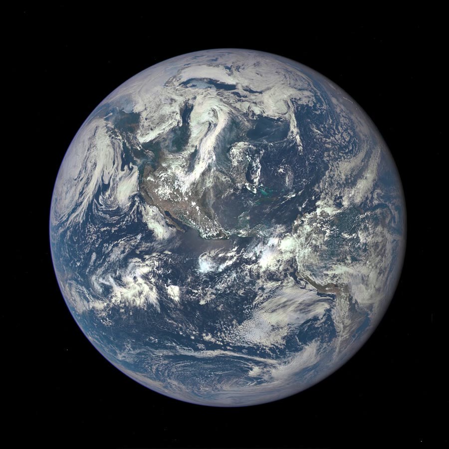
From a million miles away, the sunlit face of the Earth is a disc of blue sea, brown land and white cloud. The sunlight falls most directly on the middle of the disc, near the tropics, and grazes its edges; the tropics absorb far more energy than the polar regions. Yet the tropics do not grow hotter year after year, nor the poles colder. Winds and ocean currents carry the excess towards the poles, several petawatts of it. This chapter measures the three terms of that balance: the sunlight each latitude receives, the part it keeps and the infrared it sends back to space, and the transport that makes up the difference. A large share of the transport travels in an invisible form, as water vapour, whose latent heat is released wherever it condenses into rain.
You already know
Chapter 1 defined the insolation, the power of sunlight received per square metre of a horizontal surface at the top of the atmosphere, while the Sun is up, with at the mean distance ; gave the Sun’s altitude from its hour angle , its declination and the latitude , ; and the hour angle of sunset, (Proposition 1.16). Chapter 3 defined the Bond albedo of a planet and its equilibrium temperature. The physics volumes give the inverse-square law for light, the radiation of a black body, per square metre with (Stefan–Boltzmann), and the latent heat of a change of state. Book 2 showed that the Earth intercepts on average a quarter of the solar constant, drew the global energy budget of the Earth and checked that it balances, and described the poleward transport of heat in words.
27.1 Insolation with latitude and season
The instantaneous insolation changes from minute to minute as the Sun crosses the sky. For the climate, what counts is its sum over a day.
Definition 27.1 (Daily-mean insolation)
The daily-mean insolation at a latitude on a given day is the instantaneous insolation averaged over the 24 hours of that day, nights included, the declination of the Sun and its distance being held at their values for the day. It is a power per square metre of horizontal surface at the top of the atmosphere, in .
Holding and fixed for a day is harmless: the declination changes by at most a day, and the distance by less than .
Theorem 27.2 (Daily-mean insolation)
At latitude , on a day when the Sun’s declination is and its distance ,
where is the hour angle of sunset in radians: when ; in the polar day (); , and , in the polar night ().
Proof. The hour angle advances uniformly through in a day, so the mean over the day is the mean over . The Sun is up for , where , and the insolation is zero otherwise. Hence
which is . The bounds come from Proposition 1.16: the altitude is zero when . If that number exceeds 1 in absolute value, the Sun never crosses the horizon: when , the integrand is positive for every and the integral runs over the whole day, ; when , it is negative for every and the Sun never rises. ∎
Two special cases are worth knowing by heart. At the equator, and whatever the season:
largest at the equinoxes, at the mean distance. At a pole in its summer, and : , the Sun circling the sky at a constant altitude equal to the declination.
Proposition 27.3 (The polar summer)
On a day of declination , the daily-mean insolation at the North Pole exceeds that at the equator if and only if , that is . At the June solstice, , the ratio is .
Proof. The two special cases above share the factor ; their ratio is , which exceeds 1 when , . With the obliquity, . ∎
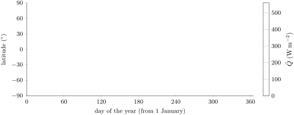
With the Earth’s orbit, the June solstice falls near aphelion, : the North Pole then receives as a daily mean, the equator . Six months later the South Pole, near perihelion, receives , more than the North Pole had in its summer: the ratio is exactly that of the two values of . The figure below shows over a whole year. The maxima are at the poles at the solstices; the dark wedges are the polar nights, bounded by the latitude ; the subsolar point, where the Sun passes overhead at noon, moves between the tropics with the declination.
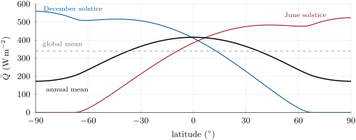
Averaging over the year gives the annual-mean insolation of each latitude (figure below): at the equator, at , at either pole. The polar summer is intense but the polar winter is dark, and over a year the equator receives times as much as a pole. The curve is the same in both hemispheres, although the southern summer is the brighter; Exercise 27.10 shows why.
Proposition 27.4 (The global mean)
At every instant, the insolation averaged over the whole sphere is . Averaged over the year as well, it is , where is the eccentricity of the orbit: for the Earth, within of .
Proof. The Earth, of radius , intercepts the sunlight crossing a disc of area , a power , which falls on the day hemisphere; spread over the whole surface , it gives the first result. The time average of over the orbit is (Exercise 27.11). ∎
27.2 Absorbed and emitted radiation
Of the sunlight a latitude receives, it reflects a fraction straight back, from clouds, snow, ice, desert and, to a lesser degree, sea; it absorbs the rest, in the air and at the surface. It also loses energy by emitting infrared radiation to space, day and night.
Definition 27.5 (Outgoing longwave radiation)
The outgoing longwave radiation (OLR) is the power of infrared radiation leaving the top of the atmosphere towards space, per square metre. The emission temperature is the temperature of a black body that would emit the same power: .
The OLR comes partly from the surface, through the air where it is transparent to infrared, and partly from the air and the cloud tops higher up. The emission temperature is a property of the radiation, not the temperature of a particular level: it is lower than that of the ground beneath, because the emitting layers are colder.
Definition 27.6 (Net radiation; radiative surplus and deficit)
The net radiation at the top of the atmosphere is
where is the local albedo, the fraction of the incoming sunlight reflected to space; all three quantities are annual means at one latitude. A latitude where has a radiative surplus; one where has a radiative deficit.
Over the whole Earth the net radiation must average almost zero, since the planet neither heats nor cools by more than a few tenths of a watt per square metre: the latest assessment puts the imbalance at , on an incoming of which are reflected (a global albedo of ) and leave as infrared.
The zonal profiles of this chapter come from a reanalysis, that is, a weather forecasting system run over the past decades, which assimilates the observations of each day and outputs a complete, consistent state of the atmosphere. The reanalysis used here, from 1948 on, gives monthly means on a grid of 94 latitudes and 192 longitudes; this chapter uses its averages over 1991–2020. Its radiation fluxes are model outputs, forecasts constrained by the observations. The figure below shows their zonal means against , so that equal widths on the axis are equal areas on the sphere.
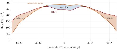
The two curves have very different shapes. The absorbed sunlight falls from near the equator to at N, by a factor of : the insolation drops, and the albedo rises from to , with the low Sun, the snow and the sea ice. The OLR falls only from to , by a factor of ; the emission temperatures are and . The OLR is even slightly lower at the equator, , than near , : the clouds of the equatorial rain belt rise high and their cold tops emit little, while the clearer subtropical skies let more infrared escape. Wherever the absorbed sunlight exceeds the OLR, the latitude has a surplus.
Example 27.7 (The reanalysis’s global budget)
Averaged over the globe, the reanalysis receives , reflects (an albedo of ), absorbs and emits : a net radiation of . The OLR is within of the assessed , but the reflection is larger than the assessed . A real imbalance of this size would cool the Earth by ; it is an error of the model, not a property of the Earth, and the transport below is computed after removing the global mean.
27.3 Meridional heat transport
Definition 27.8 (Meridional heat transport)
The meridional heat transport across the parallel of latitude is the energy carried northwards across that parallel per unit time, by the atmosphere and the ocean together, in the annual mean. It is counted positive northwards and measured in petawatts ( = ).
Proposition 27.9 (Transport from the net radiation)
If the energy stored in each latitude band does not change from year to year, then for an Earth of radius ,
and is extreme at the latitudes where changes sign.
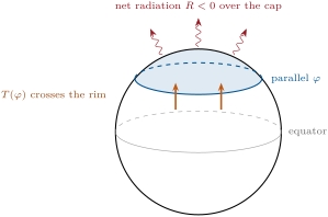
Proof. Take the polar cap south of the parallel as a control volume, from the bottom of the ocean to the top of the atmosphere (figure below). Energy enters or leaves it in only two ways: as radiation at the top, a net power , and by the transport across its rim, (a northward transport leaves the southern cap). The band between and has area . With no change of storage, the sum is zero: . Applied to the whole Earth (, no rim), the same balance gives over the sphere, whence the second form. Differentiating, , which vanishes where changes sign. ∎
Applied to the reanalysis, with its global mean of subtracted from at every latitude, the proposition gives the curve below. The transport is northward in the northern hemisphere and southward in the southern one, always towards the pole. It peaks at near N and near S, where minus its mean changes sign; across N it is . It is small at the equator, where the surplus of each hemisphere is exported to its own pole.
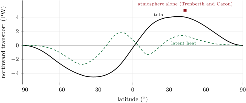
The square on the figure is a warning. A study of the years 1985–1989, when a satellite experiment measured the radiation at the top of the atmosphere reliably, computed the transport of the atmosphere from the winds, temperatures and moisture of two reanalyses: the atmosphere alone carries at N, more than this reanalysis’s for the atmosphere and the ocean together. The same study found that the model-generated fluxes of the reanalysis agree less well with independent ocean estimates than fluxes derived from the observations. Once the global mean is removed, the transport depends only on how varies with latitude, and this reanalysis’s net radiation varies too little from the tropics to the poles. The shape of the curve, its peaks in the mid-latitudes and its near-symmetry, can be trusted; its height falls at least a fifth short.
Who carries the heat? The same study finds that the ocean carries more than the atmosphere only between the equator and N; at , where the total transport peaks in each hemisphere, the atmosphere carries of it in the north and in the south. The ocean’s share is the subject of Chapter 29, the atmosphere’s of Chapter 28.
Method 27.10 (Transport from zonal bands)
- Divide the cap poleward of the latitude of interest into bands; for each, take the mean insolation , albedo and OLR.
- Compute the net radiation of each band, , and subtract the global mean of if it is not zero.
- Compute the area of each band, , with .
- The transport across the rim is minus the net power of the cap, , positive towards the pole; divide by for petawatts.
27.4 Latent and sensible heat
The surface of the Earth absorbs most of the sunlight, but the atmosphere radiates most of the infrared to space. The surface hands energy to the air in three ways: by its own infrared radiation, by warming the air in contact with it, and by evaporating water, whose latent heat is released wherever the vapour condenses. That place may be thousands of kilometres away: the latent heat travels with the wind.
Definition 27.11 (Latent and sensible heat fluxes; Bowen ratio)
The latent heat flux is the power per square metre that the surface loses by evaporation: the evaporation rate , in , times the latent heat of vaporisation . The sensible heat flux is the power per square metre that the surface passes to the air by conduction and turbulence, warming it. Both are counted positive upwards. Their ratio is the Bowen ratio.
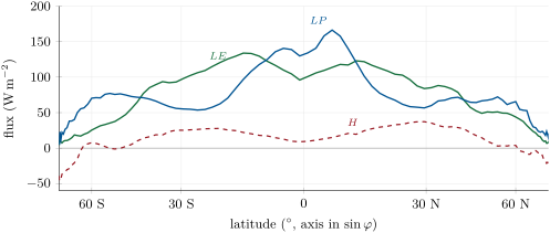
Near , . The Bowen ratio is small over the sea and over wet ground, where water is plentiful, and large over dry land. In the reanalysis it is at the equator, at N, the latitude of the great hot deserts, and negative at N, where the snow and ice surfaces are colder than the air above them in the annual mean, so that the sensible heat flows downwards. Averaged over the globe, the reanalysis gives and , a Bowen ratio of ; the assessed values are and , a ratio of .
Book 2 turned the latent heat flux into a depth of water evaporated each year. The converse turns a rainfall, which a gauge can collect, into an energy flux.
Proposition 27.12 (Precipitation as an energy flux)
A precipitation rate of of water per year releases in the atmosphere, where its vapour condensed, a mean power of
Proof. A layer of water deep has a mass of per square metre. Condensing the vapour that forms it releases ; a year of days lasts . ∎
Example 27.13 (The water cycle as an energy flux)
The global water cycle brings cubic kilometres of rain and snow to the ocean every year and to the land: spread over the Earth’s , per year, which releases by Proposition 27.12. The reanalysis rains a day, a year, . Both are close to the assessed latent heat flux of , whose uncertainty range is : over the years, the water that evaporates comes down again, and the latent heat taken from the surface is all given to the air.
The balance holds for the globe, not for each latitude, and the difference is a transport (figure below). In the subtropics the sea evaporates more water than falls there: exceeds , the latent heat of the precipitation. The equatorial rain belt and the mid-latitudes receive more rain than they evaporate. Between the two, the vapour is carried by the wind, and with it latent heat. By the argument of Proposition 27.9, applied to the integral of , the reanalysis carries of latent heat northwards across N, a third of its total transport there; the latent transport is drawn dashed on the transport figure above.
27.5 The surface energy budget
The global budget drawn in Book 2 can be read as one equation for the surface.
Proposition 27.14 (Surface energy balance)
Let be the net radiation at the surface, absorbed sunlight plus infrared received from the air minus infrared emitted, and the power per square metre that goes into the ground or the ocean below. Then, per square metre,
In the global mean, , of which go into evaporation, into the sensible heat flux, and , within the rounding of the figures, into the ocean and the ground.
Proof. Take as a system a thin layer at the surface, with no heat capacity of its own. Energy reaches it only as radiation (, net) and leaves it only as the latent and sensible heat fluxes upwards and the conduction or mixing downwards; the balance is the equation. The numbers are the assessed global means. ∎
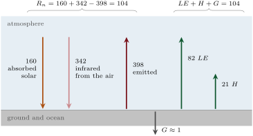
The latent heat flux, four fifths of , is the larger of the two non-radiative terms by far: over the globe, the surface cools mainly by evaporating water. The small is the climate system’s heating, the of the budget at the top of the atmosphere; nine tenths of it is stored in the ocean.
Remark 27.15 (Local and global)
At a single place, is far from small: it is large and positive by day and in summer, negative by night and in winter, and it averages out only over a day or a year. Over the ocean, the heat stored in the mixed layer can also be carried away sideways by the currents: the local balance must then include the ocean’s transport, as the balance of a latitude band includes the atmosphere’s.
27.6 Exercises
Exercise 27.1 ★
(a) Compute with . (b) On the day of the March equinox, the daily-mean insolation at the equator is . Deduce and on that day. (c) At the June solstice, and . Compute the daily-mean insolation at the equator.
Solution
Solution of Exercise 27.1.
(a) . (b) At the equator on an equinox , so and : the Earth is closer to the Sun than its mean distance. (c) .
Exercise 27.2 ★
The annual-mean insolation is at the equator and at the poles; the global mean is . (a) By what factor does the equator exceed the poles? (b) The annual mean equals the global mean at N and S. What fraction of the Earth’s surface lies between these two parallels? (c) Why does this make the annual-mean curve look more favourable to the high latitudes than the Earth’s surface really is?
Solution
Solution of Exercise 27.2.
(a) . (b) The zone between the parallels has the area , a fraction of the sphere: , . (c) On an axis in latitude, the bands near the poles look as wide as those near the equator, but they cover much less area: the zone poleward of is only of the surface. Against , the tropics fill most of the axis.
Exercise 27.3 ★
In the reanalysis the OLR is near the equator, at N and in the global mean. (a) Compute the three emission temperatures. (b) Over the same latitudes, the absorbed sunlight falls from to . Compare the two ratios. (c) What does the comparison imply for the net radiation?
Solution
Solution of Exercise 27.3.
(a) : , and . (b) Absorbed sunlight: ; OLR: . (c) The net radiation follows the absorbed sunlight: positive and large in the tropics, strongly negative at high latitudes. The OLR, which varies little, does not offset the fall of the absorbed sunlight.
Exercise 27.4 ★
The reanalysis’s global mean precipitation is a day. (a) Convert it to metres per year. (b) Compute the latent heat it releases, in , with Proposition 27.12. (c) Compare with the reanalysis’s own global latent heat flux, , and explain why the two should agree over many years.
Solution
Solution of Exercise 27.4.
(a) , a year. (b) . (c) The reanalysis’s is larger. Over many years the atmosphere cannot keep accumulating water vapour: all the water evaporated comes down again, so and must be equal in the global mean. The difference is an imbalance of the model, like its radiative imbalance.
Exercise 27.5 ★★
(a) At the June solstice (, ), compute the daily-mean insolation at the North Pole. (b) At the December solstice, ; compute it at the South Pole and the ratio of the two. (c) The Sun stands only above the horizon at the pole: explain how the pole can still beat the equator.
Solution
Solution of Exercise 27.5.
(a) . (b) ; the ratio is . (c) The pole has sunlight 24 hours out of 24 at a constant altitude, so its mean over the day is . At the equator the Sun is high at noon but down half the time; the mean of over the 24 hours is . The ratio is (Proposition 27.3).
Exercise 27.6 ★★
At N, compute the hour angle of sunset, the length of the day and the daily-mean insolation (a) at the June solstice, with , ; (b) at the December solstice, with , . (c) What share of the ratio between the two comes from the distance to the Sun?
Solution
Solution of Exercise 27.6.
(a) , ; the day lasts ; . (b) , , ; . (c) The ratio is . The distance contributes : it works against the northern summer. The geometry, the altitude of the Sun and the length of the day, contributes , all of the seasonal contrast and more.
Exercise 27.7 ★★
The reanalysis gives the following zonal means ():
| latitude | N | N | N | |
| 96.0 | 96.4 | 52.4 | 23.7 | |
| 8.9 | 36.1 | 17.7 |
(a) Compute the Bowen ratio at each latitude. (b) Which latitude has the largest ratio? What kind of surface explains it? (c) Interpret the sign of at N.
Solution
Solution of Exercise 27.7.
(a) : at the equator, at N, at N, at N. (b) N: the zonal mean includes the great hot deserts, dry land with little water to evaporate, where the heated ground warms the air instead. (c) means that heat flows from the air to the surface: in the annual mean the snow and sea ice are colder than the air above them, which is warmed by air brought from lower latitudes.
Exercise 27.8 ★★
The assessed global budget at the top of the atmosphere is incoming, reflected, emitted; the reanalysis gives , and . (a) Compute the two albedos and the two net radiations. (b) Which term explains most of the reanalysis’s imbalance? (c) Show that if the global mean of were not removed, Proposition 27.9 would leave a transport of at the North Pole, and explain why that is impossible.
Solution
Solution of Exercise 27.8.
(a) Assessed: , (the rounded). Reanalysis: , with these rounded terms, with the unrounded ones of Example 27.7. (b) The reanalysis absorbs against , less, because it reflects more; its OLR is only lower. The excess reflection explains the imbalance. (c) Integrating from the South Pole to the North Pole gives the global integral, . A transport across the North Pole is impossible: there is nothing beyond it, the parallel is a point. The proposition holds only if , which the steady state requires.
Exercise 27.9 ★★
In the reanalysis, the belt between S and N has a mean net radiation, after removal of the global mean, of . (a) Compute the area of the belt and its total surplus in petawatts. (b) If the two hemispheres exported the surplus equally, how much would cross each of the parallels N and S? (c) The reanalysis gives northwards across N and southwards across S. What does the difference say?
Solution
Solution of Exercise 27.9.
(a) The area is , half the Earth; the surplus is . (b) across each parallel. (c) The two add up to , the surplus, but they are unequal: the southern hemisphere exports more than the northern one. The surplus is not shared at the equator: in this reanalysis of the northern tropics’ surplus crosses the equator southwards.
Exercise 27.10 ★★★
The daily-mean insolation depends on the latitude, the declination and the factor . (a) With Kepler’s second law, constant, where is the Sun’s ecliptic longitude, show that the energy a latitude receives while advances by does not depend on . (b) Deduce that the annual-mean insolation at latitude equals that at , although the southern summer is brighter. (c) In the orbit model of this chapter, the Sun takes days from the March to the September equinox and days back. Explain how these numbers fit (b).
Solution
Solution of Exercise 27.10.
(a) Write the daily mean as , with the bracket of Theorem 27.2 times . During the energy received per square metre is , and , so : the factor cancels. (b) Over a year the energy is . The formula is unchanged when and change sign together, , and , since . Shifting by in the integral shows that receives the same energy as . (c) The northern spring and summer last days longer, because the Earth is near aphelion and moves slowly then; the southern summer is brighter but shorter. By (a), the two effects cancel exactly.
Exercise 27.11 ★★★
(a) Using Kepler’s second law in the form and the area of the ellipse, over a period , show that the time average of over an orbit is . (b) Complete the proof of Proposition 27.4. (c) With , compute the global annual mean and its difference from .
Solution
Solution of Exercise 27.11.
(a) , and . (b) The instantaneous global mean averages to . (c) , or above .
Exercise 27.12 ★★★
The reanalysis gives a total transport of across N and across N. (a) Using the partition of Trenberth and Caron at N (atmosphere ), split the reanalysis’s total into an atmospheric and an oceanic part. (b) The same study finds for the atmosphere alone at N. What does this say about the reanalysis? (c) Removing the global mean of does not cure this error. Why not?
Solution
Solution of Exercise 27.12.
(a) Atmosphere , ocean . (b) The atmosphere alone is found to carry more, , than the reanalysis’s atmosphere and ocean together, : the reanalysis’s total transport is short by at least a fifth (). Its net radiation varies too little between the tropics and the poles. (c) Removing a constant from makes its global integral zero but leaves its variation with latitude unchanged; the error lies in that variation, in the albedo of the model’s clouds and surfaces at each latitude, not only in the global mean.
27.7 Problem: How much heat crosses the 40th parallel?
Problem 27.1
Weekend problem — the energy budget of the cap north of N
The cap of the Earth north of N, which holds most of Europe, Russia and Canada, radiates more energy to space than it absorbs from the Sun. This problem measures the deficit, and so the heat that the atmosphere and the ocean bring across the 40th parallel. Use , , , . The band data are the reanalysis’s means for 1991–2020.
Part I — Sunlight north of N. On the June solstice and ; on the December solstice and ; on the March equinox and .
- Compute the daily-mean insolation at N on the three days.
- Compute it at N on the same three days.
- In June, N receives more than N. Explain why, with the hour angles of sunset.
- By integrating the theorem over the year, one finds annual means of , , , and at , , , and N. Compare with the band insolation of the table in Part II and give two reasons for the differences.
- The reanalysis’s global mean insolation is . What value of does it imply?
- Compute the area of the cap north of N and the fraction of the Earth’s surface it covers.
Part II — Absorbed and emitted. The reanalysis gives, for five bands of the cap:
| band | – | – | – | – | – |
| () | 308.4 | 262.4 | 217.3 | 188.7 | 176.1 |
| albedo | 0.358 | 0.393 | 0.426 | 0.510 | 0.576 |
| OLR () | 226.1 | 210.3 | 201.3 | 197.4 | 191.6 |
- Compute the absorbed solar radiation of each band.
- Compute the net radiation of each band. Which band has the largest deficit?
- Compute the emission temperature of each band.
- From – to –, by what factor does the absorbed sunlight fall, and by what factor the OLR?
- Give two reasons why the albedo increases towards the pole.
- Why does the OLR vary so much less than the absorbed sunlight?
Part III — The net radiation of the cap.
- Compute the area of each band and check that they add up to the area of Question 6.
- Compute the net radiative power of each band and of the whole cap, in petawatts.
- Compute the mean albedo of the cap, weighting each band by its incoming sunlight, and compare it with the reanalysis’s global albedo of .
- The reanalysis’s global mean net radiation is . What would this mean if it were real? Compare with the assessed imbalance of .
- Subtract this global mean from the net radiation of each band and compute again the net power of the cap.
- Explain, with Proposition 27.9, why the corrected deficit of the cap must be brought in across the 40th parallel.
Part IV — The transport and its latent share. Over the cap the reanalysis gives a mean latent heat flux of and a mean precipitation of a day; over the globe, the mean of is .
- Compute the transport across N, in petawatts.
- Compute the latent heat released by the cap’s precipitation, in , and compare it with .
- Removing the global mean of , compute the latent heat brought into the cap as water vapour, in petawatts.
- What fraction of the transport across N is latent heat?
- Taking the share of the atmosphere found by Trenberth and Caron at N, , as valid at N, split the transport into latent heat, the rest of the atmospheric transport, and the ocean.
- The same study finds for the atmosphere alone at N. Is your answer an upper or a lower bound of the truth?
- How much heat crosses the 40th parallel north, in petawatts?
Solution
Solution of Problem 27.1.
- June: , , . December: , . March: , .
- June: , polar day, : . December: polar night, . March: .
- At N the Sun does not set (, 24 hours) while at N it shines for . Its altitude is lower, between and , but the term , which grows with the day length and the latitude, wins.
- The band values exceed the central values by , , , and . First, the reanalysis uses a slightly larger solar irradiance (Question 5), more. Second, a band mean is not the value at the centre: the equatorward half of each band has more area and more sunlight than the poleward half.
- By Proposition 27.4, , more than .
- , a fraction of the Earth.
- : , , , , .
- : , , , , . All five bands are in deficit; the polar band – has the largest.
- : , , , , .
- Absorbed: ; OLR: .
- The Sun is lower, and light arriving at a grazing angle is reflected more by clouds and water; snow and sea ice, bright surfaces, cover more of the ground and the sea towards the pole.
- The OLR goes as , and varies by only , , across the cap: the high latitudes are kept much warmer than their sunlight alone would allow, by the heat brought from the south.
- In : , , , , ; the sum is .
- : , , , , ; the cap: .
- , against for the globe.
- : the Earth would be losing heat at that rate and cooling. The assessed imbalance is , eighteen times smaller and of the opposite sign: the reanalysis’s imbalance is a model error.
- Corrected : , , , , ; powers , , , , ; the cap: , a mean deficit of .
- The cap’s energy does not change from year to year, so what it loses at the top of the atmosphere must enter it, and the only way in is across the 40th parallel: .
- , northwards.
- , more than : more water falls on the cap than evaporates from it; the difference arrives as vapour.
- ; times the area of the cap: . The atmosphere brings of latent heat across N.
- : a third.
- Ocean ; atmosphere , of which latent and carried as sensible heat and potential energy of the air.
- A lower bound. The reanalysis’s total at N, , is less than the atmosphere alone in the study, ; the true total is larger.
- About , , according to the reanalysis’s radiation, a third of it as latent heat; the true value is larger still.