20Erosion and Transport

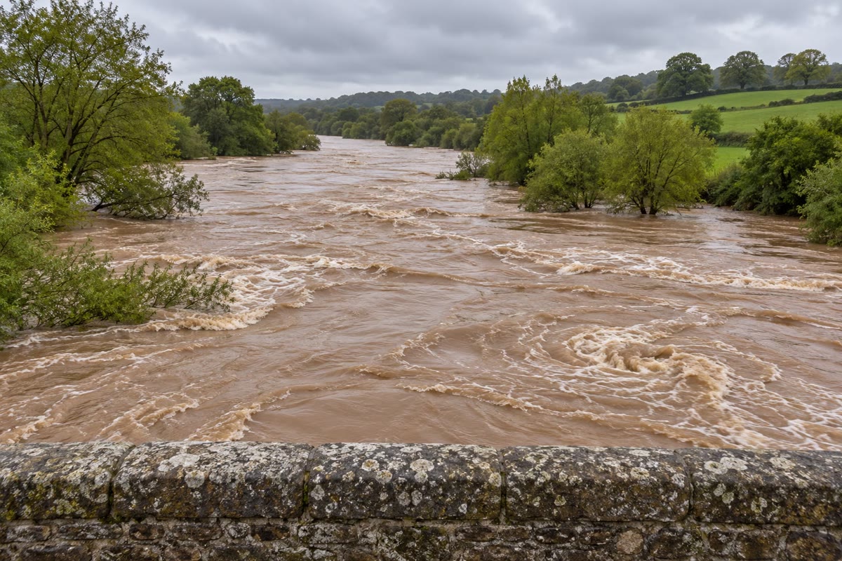
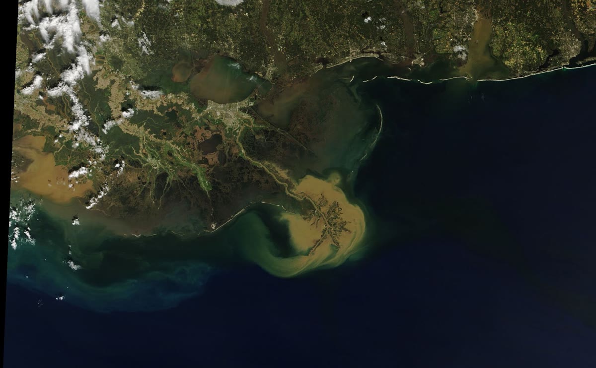
After a storm the river under the bridge runs brown. The water that was clear the day before is thick with mud, swirls around the piers and carries branches, and on the bed, unseen, pebbles knock against each other as they roll. Each second the flood takes tonnes of the land with it. Downstream, behind a dam, the same mud settles in the still water of the reservoir, which loses a little of its volume every year; farther still, at the river’s mouth, it spreads into the sea as a brown plume that can be seen from space. This chapter puts numbers on that journey: how much a river carries and in what forms, how fast a grain sinks, what current it takes to set it moving, and how fast, in the end, a whole landscape is worn away.

You already know

Erosion is the wearing-away of the land and the carrying-away of the pieces; deposition is their laying-down where the carrier slows (Book 1, grade 5). A river carries its sediment load as bed load, suspended load and dissolved load; the denudation rate of a region is the thickness of rock removed from it per unit time, in metres per million years; when erosion removes a thickness $e$ of crust, isostatic rebound lets the surface go down by only $e(1 - \rho_c/\rho_m)$ (Book 2, grade 12). The discharge of a river is the volume of water that passes a cross-section per unit time, and its drainage basin the area that supplies it (Book 2, grade 10). In Airy isostasy the crust floats on the mantle with a root proportional to its relief (Proposition 11.5). The hydrolysis of silicates sends ions and dissolved silica to the rivers (Definition 19.3). The dynamic viscosity $\mu$ of a fluid measures its resistance to shearing, and the kinematic viscosity is $\nu = \mu/\rho$; a sphere of diameter $d$ moving slowly at the speed $w$ through a fluid feels the drag $3\pi\mu d w$ (Stokes’ law); the Reynolds number $w d/\nu$ compares inertia with viscous forces, and the flow around the sphere is smooth while it stays small (the physics books).

20.1 Solute and particle fluxes

A river removes the land in two ways: as matter in solution, the products of chemical weathering, and as solid grains, the products of physical weathering and the insoluble residues of chemical weathering. The two travel differently, and the grains themselves travel in two ways.

Definition 20.1 (Dissolved load, suspended load, bed load)

The load of a river is the matter it carries past a cross-section, in three parts that differ by how they travel. The dissolved load is the matter in solution, ions and dissolved silica, which moves with the water at its own speed. The suspended load is made of grains held up within the flow by its turbulence, mostly clay, silt and fine sand, which move at nearly the speed of the water and seldom touch the bed. The bed load is made of grains that roll, slide or hop along the bed, in frequent contact with it, much more slowly than the water.

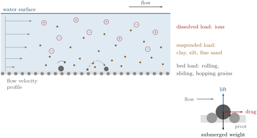
The boundary between the two solid loads is not fixed by the grain size: it depends on the flow. A flood that carries sand in suspension leaves it on the bed, as bed load, when it wanes; the finest clay, on the other hand, stays in suspension in almost any current and is hardly ever found on the bed of a flowing river. Each load is measured as a flux, a mass per unit time through a cross-section of the river.

Proposition 20.2 (Flux of a load)

Let $c$ be the concentration of a dissolved or suspended load (mass per unit volume of water) and $u$ the velocity of the water, both varying across the section of area $A$. (1) The instantaneous flux of the load through the section is

$$F = \iint_A c\,u\,\mathrm dA = \overline{c}_Q\,Q,$$

where $Q = \iint_A u\,\mathrm dA$ is the discharge and $\overline{c}_Q$ the mean concentration weighted by the velocity. (2) Over a period $T$ in which the discharge $Q(t)$ and the concentration $C(t)$ of the river vary, the mass carried is

$$M = \int_0^T Q\,C\,\mathrm dt = T\left(\overline{Q}\;\overline{C} + \operatorname{cov}(Q, C)\right),$$

where the bars are means over time and $\operatorname{cov}(Q, C)$ is the mean of $(Q - \overline{Q})(C - \overline{C})$. The product of the mean discharge and the mean concentration gives the right mass only if the two are uncorrelated.

The covariance matters for the suspended load. Its concentration rises steeply in floods, when the rain washes soil into the streams and the faster flow lifts grains from the bed, so $Q$ and $C$ grow together: a large part of a river’s yearly sediment passes in a few days of flood, and a sampling campaign that misses them, or a mean concentration multiplied by the mean discharge, underestimates the load. The dissolved load behaves the other way: floods dilute it, and its concentration is highest at low flow, when the river is fed by ground water that has been in long contact with the rock.

Method 20.3 (The yearly load of a river from gauging)

1. Record the discharge continuously at a gauging station.
2. Sample the water at many discharges, floods included, and measure the mass of sediment per litre (by filtering and weighing) and of each dissolved species.
3. Weight the concentrations by the discharge at the time of sampling to get the flow-weighted mean concentration, or fit the concentration as a function of the discharge and apply it to the whole record.
4. Multiply by the total volume of water of the year, or sum $Q\,C\,\Delta t$ over the record (Proposition 20.2).
5. Add the bed load, which water samplers miss, from separate measurements or as an estimated fraction.
6. For the dissolved load, remove what does not come from the rock: the salts brought by rain and, for the bicarbonate, the carbon taken from the air (Chapter 19).

The world’s rivers. Before any human influence, the rivers of the world carried an estimated $14\,\mathrm{Gt}$ of suspended sediment a year to the coastal ocean, $15.5\,\mathrm{Gt}$ with the bed load. People have changed both ends of the journey: farming and deforestation have raised soil erosion, adding about $2.3\,\mathrm{Gt}$ a year to the rivers, while reservoirs hold back sediment: the large ones trap about $20\,\%$ of the flux and the small ones another $6\,\%$, and more than $100\,\mathrm{Gt}$ of sediment now lies behind dams built mostly in the past fifty years. The net effect is a reduction: the modern flux is about $12.6\,\mathrm{Gt}$ a year.

Figures as of 2005

The figures for the suspended sediment flux, before and after human influence, come from a global model of river sediment published in 2005. Dams have been built since.

The dissolved load is smaller. A classic compilation of river analyses, made in 1963, put the dissolved matter that the rivers of the world deliver to the sea at about $3.9\,\mathrm{Gt}$ a year, about $30\,\%$ of the modern suspended flux, at a mean concentration of $120\,\mathrm{mg}$ per litre. Bicarbonate makes nearly half of it, $58\,\mathrm{mg}\,\mathrm{L}^{-1}$, followed by calcium, silica, sulfate, chloride and sodium. Part of it does not come from the rock: much of the bicarbonate carries carbon drawn from the air or the soil, and part of the chloride and sodium comes from sea salt carried by rain. Individual rivers range widely around these means.

The sediment budget of a basin. Not every grain eroded in a drainage basin reaches its outlet. Soil washed from a field may stop at the foot of the slope, sand may be stored for centuries in the floodplain and the river’s bars, and a reservoir may hold back most of what enters it. The load measured at the outlet is the balance of the budget: what is eroded on the slopes and from the banks, minus what is stored on the way, plus what is taken back from old stores. Over a few decades of gauging this balance can be far from the long-term rate of erosion, in either direction, which is one reason for the other methods of Section 20.4.

20.2 Settling velocity

A grain is denser than water and sinks. Whether a river can carry it, and where it will be deposited, depends first on how fast it sinks.

Definition 20.4 (Settling velocity)

The settling velocity $w_s$ of a grain is the constant velocity at which it falls through still water, when the drag of the water balances its submerged weight, its weight minus the buoyancy of the water it displaces.

A grain released in still water accelerates until its drag, which grows with its speed, balances its submerged weight; for a grain of sand or silt this takes a small fraction of a second, so the settling velocity is the speed at which it falls nearly all the way. With the densities $\rho_s$ of the grain and $\rho$ of the water, write $R = (\rho_s - \rho)/\rho$ for the relative submerged density.

Proposition 20.5 (Stokes settling)

A sphere of diameter $d$ and density $\rho_s$ falling slowly through water of density $\rho$ and dynamic viscosity $\mu$, under Stokes’ law, has the settling velocity

$$w_s = \frac{(\rho_s - \rho)\,g\,d^2}{18\,\mu} = \frac{R\,g\,d^2}{18\,\nu}.$$

The law holds while the grain Reynolds number $w_s d/\nu$ is below about 1, that is, for diameters below $d_1 = \left(18\,\nu^2/(R\,g)\right)^{1/3}$.

For quartz, of density $2650\,\mathrm{kg}\,\mathrm{m}^{-3}$, in water at $20\,{}^{\circ}\mathrm{C}$, of density $998.2\,\mathrm{kg}\,\mathrm{m}^{-3}$ and viscosity $1.0016\,\mathrm{mPa}\,\mathrm{s}$: $R = 1.65$, $\nu = 1.003 \times 10^{-6}\,\mathrm{m}^{2}\,\mathrm{s}^{-1}$, and with $g = 9.81\,\mathrm{m}\,\mathrm{s}^{-2}$ the limit is $d_1 = 0.104\,\mathrm{mm}$, a fine sand. Below it, Stokes’ law gives the settling velocities of silt and clay: a silt grain $10\,\text{µ}\mathrm{m}$ across sinks at $9.0 \times 10^{-5}\,\mathrm{m}\,\mathrm{s}^{-1}$, $1\,\mathrm{m}$ in about three hours; a clay particle of $2\,\text{µ}\mathrm{m}$ at $3.6 \times 10^{-6}\,\mathrm{m}\,\mathrm{s}^{-1}$, $1\,\mathrm{m}$ in $3.2$ days. Natural clay particles are flakes, not spheres, and sink still more slowly. Water $5\,\mathrm{m}$ deep, perfectly still, would take sixteen days to clear of such clay; a flowing river, whose eddies keep stirring it up, never does, which is why the finest mud travels to the sea.

Above $d_1$ the drag grows faster than in proportion to the velocity: the water flowing past the grain separates behind it into a wake, and at large Reynolds numbers the drag is proportional to the square of the velocity. Experiments on natural grains are summed up in a single formula that joins the two regimes.

Proposition 20.6 (Combined settling law)

The settling velocity of natural grains of sieve diameter $d$ is, for all sizes,

$$w_s = \frac{R\,g\,d^2}{C_1\,\nu + \sqrt{0.75\,C_2\,R\,g\,d^3}},$$

with $C_1 = 18$ and $C_2 = 1.0$.

The law is due to Ferguson and Church, who fitted it to measured settling velocities of natural sands. For small grains the square root is negligible and it reduces to Stokes’ law; for large grains the first term of the denominator is negligible and $w_s \to \sqrt{4 R g d/(3 C_2)}$, which grows only as the square root of the size. The constants depend on the shape of the grains: $C_2 = 0.4$ describes smooth spheres, larger values more angular grains, which meet more drag. The two laws part company above $0.1\,\mathrm{mm}$. For a grain of $1\,\mathrm{mm}$ the combined law gives $0.126\,\mathrm{m}\,\mathrm{s}^{-1}$, seven times less than Stokes’ law; for a pebble of $10\,\mathrm{mm}$, $0.46\,\mathrm{m}\,\mathrm{s}^{-1}$ against a meaningless $90\,\mathrm{m}\,\mathrm{s}^{-1}$ (diagram below).

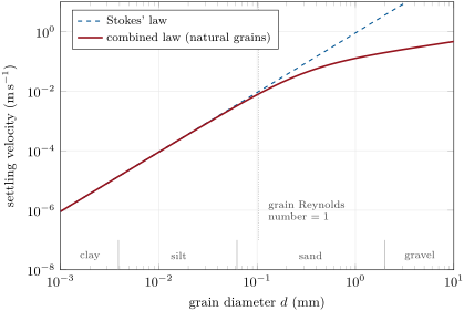
Over the range of the diagram, from the finest clay to a coarse gravel, the settling velocity spans eight orders of magnitude. This is the first reason why rivers sort their sediment: a slackening current drops its gravel at once, its sand within metres, its silt within kilometres, and carries its clay to a lake or to the sea. The grain-size classes and the sorting of sediments are the subject of the next chapter (Chapter 21).

20.3 Threshold of motion and the Hjulström diagram

A grain at rest on the bed of a river is set moving by the force of the water flowing over it. That force is measured by a stress.

Definition 20.7 (Bed shear stress, shear velocity)

The bed shear stress $\tau_b$ of a flow is the force per unit area that it exerts on its bed, parallel to the bed, in the direction of the flow. The shear velocity is $u_* = \sqrt{\tau_b/\rho}$, a velocity that measures the same stress.

The bed shear stress cannot be read from a current meter, but in a steady flow it follows from a balance of forces.

Proposition 20.8 (Depth–slope product)

In a steady, uniform flow of depth $h$ down a wide channel of small slope $S$, the bed shear stress is

$$\tau_b = \rho\,g\,h\,S .$$

A river $2\,\mathrm{m}$ deep on a slope of $0.001$, a metre of fall per kilometre, has $\tau_b = 998.2 \times 9.81 \times 2 \times 0.001 = 19.6\,\mathrm{Pa}$, and a shear velocity of $0.140\,\mathrm{m}\,\mathrm{s}^{-1}$. In a channel that is not wide, the banks take their share of the friction, and the depth is replaced by the hydraulic radius, the area of the section divided by its wetted perimeter (Exercise 20.5).

Forces on a grain. The flow pushes a grain of the bed by its drag and lifts it by the faster flow over its top (the inset of the first figure of this chapter). Both forces act on the area of the grain, so they scale as $\tau_b d^2$; the grain resists by its submerged weight, which scales as $(\rho_s - \rho) g d^3$. The ratio of the two is the natural measure of the flow’s strength for a given grain.

Definition 20.9 (Shields parameter, threshold of motion)

The Shields parameter of a flow of bed shear stress $\tau_b$ over grains of diameter $d$ and density $\rho_s$ is

$$\theta = \frac{\tau_b}{(\rho_s - \rho)\,g\,d}.$$

The threshold of motion of the grains is the bed shear stress, or the value $\theta_c$ of the Shields parameter, at which they begin to move.

The critical value $\theta_c$ is measured in flumes, and the measurements fall on one curve when they are plotted against a dimensionless grain size that combines the grain and the fluid.

Proposition 20.10 (Threshold curve of Soulsby and Whitehouse)

For grains of diameter $d$ on a flat bed, with $D_* = d\,\left(R\,g/\nu^2\right)^{1/3}$, the critical Shields parameter is

$$\theta_c = \frac{0.3}{1 + 1.2\,D_*} + 0.055\left(1 - e^{-0.02\,D_*}\right),$$

and the critical bed shear stress is $\tau_c = \theta_c\,(\rho_s - \rho)\,g\,d$.

For coarse grains $\theta_c$ tends to $0.055$: gravel moves when the bed shear stress reaches about a twentieth of the submerged weight of a layer of grains one diameter thick, per unit area. Formulas of sediment transport that use a constant threshold take values from $0.03$ to $0.047$, the latter in the classic bed-load formula of Meyer-Peter and Müller. For fine sand $\theta_c$ rises again, to $0.077$ at $0.1\,\mathrm{mm}$: small grains lie within the slow, viscous layer of water close to the bed and are sheltered by their neighbours. The minimum, $0.030$, falls near $0.7\,\mathrm{mm}$. In pascals the threshold always grows with the size (diagram below): $0.13\,\mathrm{Pa}$ for a sand of $0.1\,\mathrm{mm}$, $0.51\,\mathrm{Pa}$ at $1\,\mathrm{mm}$, $9.0\,\mathrm{Pa}$ at $10\,\mathrm{mm}$, $57\,\mathrm{Pa}$ for a cobble of $64\,\mathrm{mm}$.

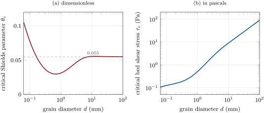
Example 20.11 (What the river moves)

In the river $2\,\mathrm{m}$ deep on a slope of $0.001$, $\tau_b = 19.6\,\mathrm{Pa}$. For grains of $20\,\mathrm{mm}$, $\theta = 19.6/(1651.8 \times 9.81 \times 0.020) = 0.060$, just above their threshold of $0.055$: they move. For grains of $40\,\mathrm{mm}$, $\theta = 0.030$, half the threshold: they stay. The river moves its bed up to coarse gravel; for sand of $1\,\mathrm{mm}$, $\theta = 1.21$, nearly forty times the threshold of $0.031$.

Into suspension. Once moving, a grain hops along the bed or is taken up into the flow, depending on whether the eddies, whose speeds are of the order of the shear velocity, can hold it up against its settling.

Proposition 20.12 (Criterion of suspension)

A grain of settling velocity $w_s$ can stay in suspension in a turbulent flow only if some eddies rise faster than it sinks. The upward velocities of the eddies being of the order of the shear velocity $u_*$, suspension begins when $u_*$ approaches $w_s$ and is fully developed when $u_*$ exceeds it; this chapter takes $u_* = w_s$ as the limit of suspension.

In the river of the example, $u_* = 0.140\,\mathrm{m}\,\mathrm{s}^{-1}$, which the combined law of settling gives to grains of $1.16\,\mathrm{mm}$: sand finer than about a millimetre travels in suspension, coarser sand and gravel as bed load. The argument goes back to Bagnold, who noted that grains of $0.1\,\mathrm{mm}$ or less are fully suspended as soon as they move, while grains larger than $1\,\mathrm{mm}$ need a bed shear stress many times their threshold. When the flood wanes and $u_*$ drops, the coarse sand falls back to the bed first.

From stress to mean velocity. What is easily measured, or estimated, in a river is its mean velocity. In a turbulent flow over a bed roughened by grains of diameter $d$, a wide channel of depth $h$ has the mean velocity $U = u_*\left(6.25 + 5.75\log_{10}(h/d)\right)$, a law established by Keulegan in 1938 from the experiments of Nikuradse and Bazin, so the threshold of motion corresponds to the critical mean velocity

and the limit of suspension, $u_* = w_s$, to $U_s = \left(6.25 + 5.75\log_{10}(h/d)\right) w_s$. Both depend on the depth, though only through a logarithm.

Threshold velocities therefore belong to one depth and one set of laws: computed for another depth, or read from other measurements, they come out different. Plotted against the grain size, their shape is robust but their values are not, and the bed shear stress, which does not depend on the depth in the same way, is the better measure of what a flow can do. The velocities are still the more intuitive, and the classic way of drawing them is a diagram.

Definition 20.13 (Hjulström diagram)

A Hjulström diagram plots the mean velocity of a flow against the diameter of the grains, on logarithmic scales, and divides the plane into the fields in which grains at rest are eroded, grains already moving are kept in transport, and moving grains are deposited.

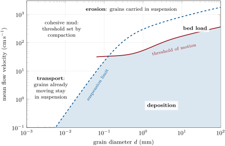
Reading the diagram. Three features carry the geology. First, the easiest grains to erode are fine sands, between about $0.06$ and $0.2\,\mathrm{mm}$, which a current of $31\text{ to }34\,\mathrm{cm}\,\mathrm{s}^{-1}$ sets moving in water $1\,\mathrm{m}$ deep; coarser grains need more, up to about $3\,\mathrm{m}\,\mathrm{s}^{-1}$ for a cobble of $64\,\mathrm{mm}$. Second, silt and clay, although they are lighter, are harder to erode than fine sand once they have settled: their particles stick together, and a compacted mud resists a current that would sweep sand away. The calculation for loose grains cannot see this, and the measured erosion velocities of muds vary with their compaction and water content, hence the hatched field. Third, the gap between erosion and deposition opens wide for the fine grains: a clay particle needs a strong current to be torn from a muddy bed, but once in the water it stays there in the gentlest flow, which is the whole history of the brown flood and of the plume in the sea.

History — Two studies of the 1930s

In 1935 Filip Hjulström, of the Geographical Institute of Uppsala, published a long study of the work of the river Fyris, in central Sweden, which contained the diagram that bears his name: erosion and deposition velocities against grain size, on logarithmic scales. Unlike earlier curves, his erosion curve had a minimum, between about $0.1$ and $0.5\,\mathrm{mm}$: loose fine sand is the easiest to erode, while coarser sand and gravel, and also silt and clay, which cohere, need stronger currents. A year later, in 1936, the engineer A. Shields, in the dissertation he defended at the Technische Hochschule of Berlin, plotted the threshold of motion as a ratio of forces, the parameter that now carries his name, against a dimensionless grain size. Hjulström’s velocities ignore the depth of the flow; Shields’ dimensionless approach does not, and it underlies the threshold formulas used today, such as the one behind the diagrams of this chapter.

20.4 Denudation rates

The loads of a river, added up over its basin, measure how fast the basin is being worn down.

Definition 20.14 (Denudation rate)

The denudation rate $D$ of a region is the mean rate at which the removal of matter, as solid grains and in solution, lowers its surface, expressed as the equivalent thickness of fresh rock per unit time, in metres per million years ($\mathrm{m}/\mathrm{Myr}$, the same as millimetres per thousand years). The mass removed per unit area and time, in tonnes per square kilometre and per year, is the specific sediment yield.

Proposition 20.15 (Denudation from river loads)

If a basin of area $A$ loses, through its outlet, the yearly masses $F_s$ of suspended load, $F_b$ of bed load and $F_d$ of dissolved load derived from its rocks, and if nothing is stored on the way, its denudation rate is

$$D = \frac{F_s + F_b + F_d}{\rho_r\,A},$$

with $\rho_r$ the density of the fresh rock. For $\rho_r = 2700\,\mathrm{kg}\,\mathrm{m}^{-3}$, a specific yield of $100\,\mathrm{t}\,\mathrm{km}^{-2}\,\mathrm{yr}^{-1}$ corresponds to $37\,\mathrm{m}/\mathrm{Myr}$.

The dissolved load counts only for the part that comes from the rock, not from the air: the carbon of the bicarbonate of silicate weathering is taken from the atmosphere, and only the cations and the silica are rock. The chemical part of denudation is not small. Where the climate is warm and wet and the relief low, it can approach or exceed the mechanical part, while in steep mountains the mechanical part dominates.

Three clocks. The denudation rate can be measured over three very different spans of time. River loads integrate years to decades, and are at the mercy of the few floods that happened, or did not happen, during the measurements. The sediment caught in a reservoir or a lake, measured by surveying its floor, integrates the decades to a century of its life. The third clock is written in the grains themselves, by cosmic rays.

Proposition 20.16 (Cosmogenic nuclides and erosion)

Suppose that a nuclide is produced in a rock by cosmic rays at the rate $P(z) = P_0\,e^{-\rho z/\Lambda}$ per unit mass, decreasing exponentially with the depth $z$ ($\rho$ the density of the rock, $\Lambda$ a constant, the attenuation length expressed as a mass per unit area), and that the surface is lowered at the steady rate $\varepsilon$. Neglecting radioactive decay, a grain that reaches the surface carries the concentration

$$N = \frac{P_0\,\Lambda}{\rho\,\varepsilon}.$$

The concentration is inversely proportional to the erosion rate: a slowly eroding surface keeps each grain near the surface for a long time and loads it with nuclides. The rate it gives is averaged over the time taken to erode the few metres in which the production is concentrated, which is from about a thousand to a million years, depending on the rate. Neglecting the decay is justified when that time is short compared with the life of the nuclide; when erosion is very slow, the decay is included and the formula becomes slightly longer.

In the lab — Beryllium-10 in river sand

The usual nuclide is beryllium-10, otherwise exceptionally rare at the surface of the Earth, made by cosmic rays in the quartz of the top few metres of rock. To measure the denudation rate of a whole basin, geochemists collect sand from the bed of its river near the outlet, on the assumption that the river mixes grains from every slope of the basin in proportion to the rate at which each is eroded. In the laboratory, the quartz is separated from the other minerals and cleaned in acids to remove the beryllium made in the air and brought down by rain; it is then dissolved, a known quantity of ordinary beryllium is added, and the beryllium is extracted. Its isotopes are counted one atom at a time with an accelerator mass spectrometer, which can find the rare beryllium-10 atoms among a vast excess of the ordinary isotope.

What the rates are. A compilation of $1599$ such measurements, published in 2011, found that bare outcrops of rock are lowered slowly: by $12\,\mathrm{m}/\mathrm{Myr}$ on average, with a median of $5.4\,\mathrm{m}/\mathrm{Myr}$ (450 outcrops). Sedimentary rock wears away faster, $20\,\mathrm{m}/\mathrm{Myr}$ on average, than metamorphic, $11\,\mathrm{m}/\mathrm{Myr}$, and igneous, $8.7\,\mathrm{m}/\mathrm{Myr}$. Whole drainage basins lose much more, $218\,\mathrm{m}/\mathrm{Myr}$ on average with a median of $54\,\mathrm{m}/\mathrm{Myr}$ ($1149$ basins): their steep slopes, landslides and river channels erode far faster than their bare summits, and a few very fast basins raise the mean four times above the median. The mean slope of a basin is the best single predictor of its rate. Basins in seismically active regions, where mountains are rising, average $367\,\mathrm{m}/\mathrm{Myr}$, against $182\,\mathrm{m}/\mathrm{Myr}$ in quiet regions; polar basins, scoured by glaciers, $537\,\mathrm{m}/\mathrm{Myr}$; arid basins $100\,\mathrm{m}/\mathrm{Myr}$.

Isostasy slows the lowering. Removing rock from a region in isostasy lightens its columns, and the crust rises to restore the balance. With $\rho_c = 2700\,\mathrm{kg}\,\mathrm{m}^{-3}$ and $\rho_m = 3300\,\mathrm{kg}\,\mathrm{m}^{-3}$ (Chapter 11), the rebound formula recalled at the start of the chapter gives a lowering of only $1 - 2700/3300 = 0.18$ of the thickness removed: to bring the mean surface of a region down by $1\,\mathrm{m}$, erosion must remove $5.5\,\mathrm{m}$ of rock. The time to wear down a mountain range is thus more than five times what its height divided by its denudation rate suggests, and the rocks now at the surface of old, worn-down ranges once lay many kilometres deep. And since the rebound follows the mean thickness removed, not its distribution, a range whose valleys are cut deeply while its peaks are barely touched rises as a whole: its peaks go up, although nothing has been added to them (Exercise 20.11).

Rates change. A denudation rate measured today is not a constant of the landscape. As relief and slopes decrease, so does the rate, and an old, lowered range is worn ever more slowly; conversely, a range that is being uplifted, or a climate that changes, raises it. A time computed from today’s rate is a first estimate, not a prediction.

20.5 Exercises

Exercise 20.1 ★

A river has a mean discharge of $500\,\mathrm{m}^{3}\,\mathrm{s}^{-1}$ and carries, as a flow-weighted mean, $0.4\,\mathrm{g}$ of suspended sediment per litre. Compute its suspended flux in kilograms per second and in millions of tonnes a year (take a year of $365.25$ days).

Solution

Solution of Exercise 20.1.

$0.4\,\mathrm{g}\,\mathrm{L}^{-1}$ is $0.4\,\mathrm{kg}\,\mathrm{m}^{-3}$, so the flux is $500 \times 0.4 = 200\,\mathrm{kg}\,\mathrm{s}^{-1}$. A year of $365.25$ days lasts $3.156 \times 10^{7}\,\mathrm{s}$, so the yearly flux is $6.31 \times 10^{9}\,\mathrm{kg}$, or $6.31\,\mathrm{Mt}$.

Exercise 20.2 ★

With Stokes’ law, compute the settling velocity of a quartz silt grain $30\,\text{µ}\mathrm{m}$ across in water at $20\,{}^{\circ}\mathrm{C}$ ($R = 1.6548$, $\nu = 1.0034 \times 10^{-6}\,\mathrm{m}^{2}\,\mathrm{s}^{-1}$, $g = 9.81\,\mathrm{m}\,\mathrm{s}^{-2}$), check that its grain Reynolds number is small, and compute the time it takes to sink through $2\,\mathrm{m}$ of still water.

Solution

Solution of Exercise 20.2.

$w_s = R g d^2/(18\nu) = 1.6548 \times 9.81 \times (30 \times 10^{-6})^2/(18 \times 1.0034 \times 10^{-6}) = 8.09 \times 10^{-4}\,\mathrm{m}\,\mathrm{s}^{-1}$, about $0.8\,\mathrm{mm}$ a second. Its grain Reynolds number is $w_s d/\nu = 8.09 \times 10^{-4} \times 30 \times 10^{-6}/1.0034 \times 10^{-6} = 0.024$, far below 1: Stokes’ law applies. It sinks through $2\,\mathrm{m}$ in $2/8.09 \times 10^{-4} = 2472\,\mathrm{s}$, about $41\,\mathrm{min}$.

Exercise 20.3 ★

A wide stream $0.5\,\mathrm{m}$ deep flows on a slope of $4 \times 10^{-4}$. Compute its bed shear stress, with $\rho = 998.2\,\mathrm{kg}\,\mathrm{m}^{-3}$, and the Shields parameter of the flow for quartz grains of $1\,\mathrm{mm}$ and of $10\,\mathrm{mm}$ ($\rho_s = 2650\,\mathrm{kg}\,\mathrm{m}^{-3}$). The critical values are $0.0314$ at $1\,\mathrm{mm}$ and $0.0556$ at $10\,\mathrm{mm}$: which grains move?

Solution

Solution of Exercise 20.3.

$\tau_b = \rho g h S = 998.2 \times 9.81 \times 0.5 \times 4 \times 10^{-4} = 1.96\,\mathrm{Pa}$. With $(\rho_s - \rho) g = 1651.8 \times 9.81 = 16\,204\,\mathrm{N}\,\mathrm{m}^{-3}$: for $1\,\mathrm{mm}$, $\theta = 1.96/(16204 \times 0.001) = 0.121$, nearly four times the threshold of $0.0314$, so the sand moves; for $10\,\mathrm{mm}$, $\theta = 0.0121$, a fifth of the threshold of $0.0556$, so the gravel stays. The stream carries its sand over a gravel bed that does not move.

Exercise 20.4 ★

The modern flux of suspended sediment to the ocean is about $12.6\,\mathrm{Gt}$ a year, the dissolved flux about $3.9\,\mathrm{Gt}$ a year, at a mean concentration of $120\,\mathrm{mg}\,\mathrm{L}^{-1}$. (a) What is the ratio of the suspended to the dissolved flux? (b) Before human influence the suspended flux was $14\,\mathrm{Gt}$ a year: what masses do the large reservoirs ($20\,\%$) and all reservoirs ($26\,\%$) trap? (c) What yearly volume of river water do the dissolved flux and its concentration imply? What is then the mean concentration of suspended sediment, in grams per litre?

Solution

Solution of Exercise 20.4.

(a) $12.6/3.9 = 3.2$: the rivers carry about three times more in suspension than in solution. (b) Large reservoirs: $0.20 \times 14 = 2.8\,\mathrm{Gt}$ a year; all of them: $0.26 \times 14 = 3.64\,\mathrm{Gt}$ a year. (c) The dissolved flux is $3.9 \times 10^{15}\,\mathrm{g}$ a year at $120\,\mathrm{g}\,\mathrm{m}^{-3}$, so the water carrying it is $3.9 \times 10^{15}/120 = 3.25 \times 10^{13}\,\mathrm{m}^{3}$, about $32\,500\,\mathrm{km}^{3}$ a year. The suspended load in that water is $1.26 \times 10^{16}\,\mathrm{g}/3.25 \times 10^{16}\,\mathrm{L} = 0.39\,\mathrm{g}\,\mathrm{L}^{-1}$.

Exercise 20.5 ★★

In a channel of finite width, the depth–slope product becomes $\tau_b = \rho g R_h S$, with the hydraulic radius $R_h$, the area of the section divided by its wetted perimeter. (a) Compute $R_h$ for a rectangular channel $10\,\mathrm{m}$ wide and $2\,\mathrm{m}$ deep. (b) Compare the bed shear stress on a slope of $0.001$ with that of a very wide channel of the same depth. (c) Show that $R_h \to h$ when the width grows.

Solution

Solution of Exercise 20.5.

(a) The section has the area $10 \times 2 = 20\,\mathrm{m}^{2}$ and the wetted perimeter $10 + 2 \times 2 = 14\,\mathrm{m}$, so $R_h = 20/14 = 1.43\,\mathrm{m}$. (b) $\tau_b = 998.2 \times 9.81 \times 1.43 \times 0.001 = 14.0\,\mathrm{Pa}$, against $19.6\,\mathrm{Pa}$ for a very wide channel $2\,\mathrm{m}$ deep: the ratio is $R_h/h = 0.714$, the banks taking the rest of the friction. (c) For a rectangular channel of width $b$, $R_h = bh/(b + 2h) = h/(1 + 2h/b)$, which tends to $h$ when $b$ grows.

Exercise 20.6 ★★

(a) Show from Proposition 20.5 that the limit $d_1$ of Stokes’ law is proportional to $\nu^{2/3}$. (b) At $10\,{}^{\circ}\mathrm{C}$ the viscosity of water is $1.3059\,\mathrm{mPa}\,\mathrm{s}$ and its density $999.7\,\mathrm{kg}\,\mathrm{m}^{-3}$; compute $d_1$ for quartz, knowing that it is $0.104\,\mathrm{mm}$ at $20\,{}^{\circ}\mathrm{C}$, where $\nu = 1.0034 \times 10^{-6}\,\mathrm{m}^{2}\,\mathrm{s}^{-1}$ (neglect the small change of $R$). (c) By what factor does a quartz silt grain of $50\,\text{µ}\mathrm{m}$ settle more slowly at $10\,{}^{\circ}\mathrm{C}$ than at $20\,{}^{\circ}\mathrm{C}$? What does this mean for a river in winter?

Solution

Solution of Exercise 20.6.

(a) $d_1 = \left(18\nu^2/(Rg)\right)^{1/3} = (18/(Rg))^{1/3}\,\nu^{2/3}$, and $R$ and $g$ do not depend on the viscosity. (b) $\nu = 1.3059 \times 10^{-3}/999.7 = 1.306 \times 10^{-6}\,\mathrm{m}^{2}\,\mathrm{s}^{-1}$ at $10\,{}^{\circ}\mathrm{C}$, against $1.0034 \times 10^{-6}\,\mathrm{m}^{2}\,\mathrm{s}^{-1}$ at $20\,{}^{\circ}\mathrm{C}$: the ratio is $1.302$, and $1.302^{2/3} = 1.192$, so $d_1 = 0.104 \times 1.192 = 0.124\,\mathrm{mm}$. (c) In the Stokes range $w_s$ is inversely proportional to $\nu$: the grain settles $1.302$ times more slowly, about $30\,\%$. Cold water holds fine sediment in suspension longer: a river in winter carries its silt somewhat farther for the same flow.

Exercise 20.7 ★★

For quartz grains of $0.1\,\mathrm{mm}$, $0.5\,\mathrm{mm}$ and $2\,\mathrm{mm}$ in water at $20\,{}^{\circ}\mathrm{C}$, compute the settling velocity by Stokes’ law and by the combined law, and the ratio of the two. Explain the trend.

Solution

Solution of Exercise 20.7.

With $R g/(18\nu) = 8.99 \times 10^{5}\,\mathrm{m}^{-1}\,\mathrm{s}^{-1}$ and the combined law:

$d$	Stokes ($\mathrm{m}\,\mathrm{s}^{-1}$)	combined ($\mathrm{m}\,\mathrm{s}^{-1}$)	ratio
$0.1\,\mathrm{mm}$	$8.99 \times 10^{-3}$	$7.53 \times 10^{-3}$	$1.19$
$0.5\,\mathrm{mm}$	$0.225$	$0.0711$	$3.16$
$2\,\mathrm{mm}$	$3.60$	$0.197$	$18.3$

The ratio grows with the size, because the grain Reynolds number grows: Stokes’ law, valid only for small Reynolds numbers, increases as $d^2$, while the drag of the wake slows the coarse grains to a velocity that grows only as $\sqrt d$.

Exercise 20.8 ★★

(a) Compute, with the curve of Soulsby and Whitehouse, the critical Shields parameter and the critical bed shear stress for quartz grains of $0.2\,\mathrm{mm}$ and $20\,\mathrm{mm}$. (b) What depth of water, flowing steadily in a wide channel on a slope of $0.002$, reaches each threshold?

Solution

Solution of Exercise 20.8.

(a) $(Rg/\nu^2)^{1/3} = 25\,263\,\mathrm{m}^{-1}$. At $0.2\,\mathrm{mm}$, $D_* = 5.05$ and $\theta_c = 0.3/7.06 + 0.055(1 - e^{-0.101}) = 0.0425 + 0.0053 = 0.0478$; $\tau_c = 0.0478 \times 16204 \times 2 \times 10^{-4} = 0.155\,\mathrm{Pa}$. At $20\,\mathrm{mm}$, $D_* = 505$ and $\theta_c = 0.3/607 + 0.055(1 - e^{-10.1}) = 0.0005 + 0.0550 = 0.0555$; $\tau_c = 0.0555 \times 16204 \times 0.02 = 18.0\,\mathrm{Pa}$. (b) $h = \tau_c/(\rho g S)$ with $\rho g S = 19.58\,\mathrm{Pa}\,\mathrm{m}^{-1}$: $7.9\,\mathrm{mm}$ of water moves the fine sand, $0.92\,\mathrm{m}$ the gravel.

Exercise 20.9 ★★

A basin of $2000\,\mathrm{km}^{2}$ exports each year $0.6\,\mathrm{Mt}$ of suspended and bed load and $0.2\,\mathrm{Mt}$ of rock-derived dissolved load. Compute its specific yield and its denudation rate for a rock density of $2650\,\mathrm{kg}\,\mathrm{m}^{-3}$. How does it compare with the median of the basins measured with beryllium-10?

Solution

Solution of Exercise 20.9.

The basin loses $0.8\,\mathrm{Mt}$ = $8 \times 10^{5}\,\mathrm{t}$ a year, or $8 \times 10^{5}/2000 = 400\,\mathrm{t}\,\mathrm{km}^{-2}\,\mathrm{yr}^{-1}$. By Proposition 20.15, $D = 8 \times 10^{8}\,\mathrm{kg}/(2650 \times 2 \times 10^{9}\,\mathrm{m}^{2}) = 1.51 \times 10^{-4}\,\mathrm{m}$ a year, or $151\,\mathrm{m}/\mathrm{Myr}$. That is about three times the median of the basins measured with beryllium-10, $54\,\mathrm{m}/\mathrm{Myr}$, though below their mean of $218\,\mathrm{m}/\mathrm{Myr}$: a fairly fast basin, as in steep or tectonically active country.

Exercise 20.10 ★★★

A wide river $3\,\mathrm{m}$ deep flows on a slope of $5 \times 10^{-4}$. (a) Compute its shear velocity and its bed shear stress. (b) With Proposition 20.12 and the combined settling law, find the largest quartz grain it carries in suspension. (c) With the threshold curve, find the largest grain it moves at all. (d) Describe the bed and the load of this river.

Solution

Solution of Exercise 20.10.

(a) $u_* = \sqrt{g h S} = \sqrt{9.81 \times 3 \times 5 \times 10^{-4}} = 0.1213\,\mathrm{m}\,\mathrm{s}^{-1}$ and $\tau_b = \rho u_*^2 = 14.7\,\mathrm{Pa}$. (b) Suspension needs $w_s < u_* = 0.1213\,\mathrm{m}\,\mathrm{s}^{-1}$. The combined law gives $0.126\,\mathrm{m}\,\mathrm{s}^{-1}$ at $1\,\mathrm{mm}$; solving $w_s(d) = 0.1213$ by trial gives $d = 0.94\,\mathrm{mm}$. (c) For gravel $\theta_c \approx 0.0555$, so $\tau_c = 14.7\,\mathrm{Pa}$ for $d \approx 14.7/(0.0555 \times 16204) = 16.3\,\mathrm{mm}$; at that size the threshold curve gives $\theta_c = 0.0555$ indeed. (d) Grains coarser than about $16\,\mathrm{mm}$ stay on the bed and form a stable gravel floor; finer gravel and the sand coarser than about a millimetre travel as bed load; finer sand, silt and clay travel in suspension.

Exercise 20.11 ★★★

A plateau in isostatic equilibrium is cut by valleys until $30\,\%$ of its volume above the valley floors is removed; before the cutting it stood as a flat surface $1000\,\mathrm{m}$ above the future valley floors. Take $\rho_c = 2700\,\mathrm{kg}\,\mathrm{m}^{-3}$ and $\rho_m = 3300\,\mathrm{kg}\,\mathrm{m}^{-3}$. (a) What mean thickness of rock is removed? (b) By how much does the region rise by isostasy? (c) By how much has the mean surface been lowered? (d) What has happened to the summits that were not eroded?

Solution

Solution of Exercise 20.11.

(a) $0.30 \times 1000\,\mathrm{m} = 300\,\mathrm{m}$ of rock, averaged over the region. (b) The rebound is $300 \times 2700/3300 = 245\,\mathrm{m}$. (c) The mean surface is lowered by $300 - 245 = 55\,\mathrm{m}$ only. (d) The summits, which were not eroded, are carried up with the whole region: they now stand $245\,\mathrm{m}$ higher than before. Cutting valleys can raise the peaks of a range.

Exercise 20.12 ★★★

A reservoir of $50 \times 10^{6}\,\mathrm{m}^{3}$ receives $0.5\,\mathrm{Mt}$ of sediment a year and traps $90\,\%$ of it. The deposit, wet and loose, has a bulk density of $1300\,\mathrm{kg}\,\mathrm{m}^{-3}$. (a) What volume of the reservoir does it fill each year, and what fraction? (b) How long until half of the reservoir is filled at this rate? (c) Why does the loss of volume usually slow down as the reservoir ages?

Solution

Solution of Exercise 20.12.

(a) $0.9 \times 5 \times 10^{8}\,\mathrm{kg}/1300\,\mathrm{kg}\,\mathrm{m}^{-3} = 346\,000\,\mathrm{m}^{3}$ a year, or $0.69\,\%$ of the reservoir. (b) Half the reservoir, $25 \times 10^{6}\,\mathrm{m}^{3}$, is filled in $25 \times 10^{6}/346\,000 = 72\text{ years}$ at this rate. (c) As the reservoir fills, its volume, and so the residence time of the water, decreases, and finer grains pass through: its trapping efficiency falls. Meanwhile the older deposits are buried and compacted, expelling water, so that their bulk density rises and each tonne takes less room. Both effects slow the loss of volume as the reservoir ages.

20.6 Problem: How fast are the Varden Hills wearing away?

Problem 20.1

Weekend problem — the river of the Varden Hills, from its loads to the time it takes to wear the hills down

The river of the Varden Hills drains a basin of $80\,\mathrm{km}^{2}$ of granite, schist and sedimentary rocks. At its outlet a gauging station records a mean discharge of $1.2\,\mathrm{m}^{3}\,\mathrm{s}^{-1}$; over several years of sampling, the flow-weighted mean concentration of suspended sediment is $150\,\mathrm{mg}\,\mathrm{L}^{-1}$, and that of the dissolved load derived from the rocks, $80\,\mathrm{mg}\,\mathrm{L}^{-1}$. The bed load is estimated at $10\,\%$ of the suspended load. Take a year of $365.25$ days, a rock density of $2700\,\mathrm{kg}\,\mathrm{m}^{-3}$, quartz grains of density $2650\,\mathrm{kg}\,\mathrm{m}^{-3}$, and water at $20\,{}^{\circ}\mathrm{C}$ ($R = 1.6548$, $\nu = 1.0034 \times 10^{-6}\,\mathrm{m}^{2}\,\mathrm{s}^{-1}$, $g = 9.81\,\mathrm{m}\,\mathrm{s}^{-2}$).

Part I — The loads.

1. Express the mean discharge as a runoff, the depth of water spread over the basin each year, in millimetres.
2. Compute the yearly flux of suspended sediment, in tonnes.
3. Compute the yearly flux of rock-derived dissolved load.
4. Compute the bed load and the total load.
5. The time-averaged concentration of suspended sediment is much lower than $150\,\mathrm{mg}\,\mathrm{L}^{-1}$. Explain why, and which of the two must be multiplied by the mean discharge.
6. What share of the total does the dissolved load make? Compare with the world’s rivers, whose dissolved flux is about $3.9\,\mathrm{Gt}$ and suspended flux $12.6\,\mathrm{Gt}$ a year.

Part II — The denudation rate.

7. Compute the specific sediment yield of the basin.
8. Compute its denudation rate, in metres per million years.
9. Compare it with the median of the basins measured with beryllium-10, $54\,\mathrm{m}/\mathrm{Myr}$. Is the basin fast or slow?
10. A beryllium-10 measurement on sand from the outlet gives a rate of the same order. What spans of time do the gauging and the beryllium average over, and why can they differ?
11. Why must only the rock-derived part of the dissolved load be counted?

Part III — A reservoir. A dam is planned at the outlet, holding a reservoir of $1.5 \times 10^{6}\,\mathrm{m}^{3}$ with a mean depth of $8\,\mathrm{m}$.

12. What is the mean residence time of the water in the reservoir, in days?
13. How long does a quartz sand grain of $0.1\,\mathrm{mm}$, entering at the surface, take to settle to the bottom (combined law)?
14. Same question for a silt grain of $0.02\,\mathrm{mm}$, with Stokes’ law.
15. Same question for a clay particle of $1\,\text{µ}\mathrm{m}$. Is it trapped?
16. What is the finest grain that settles through the whole depth within the residence time?
17. Suppose that the bed load and $70\,\%$ of the suspended load are trapped, the rest being finer clay, and that the deposit has a bulk density of $1300\,\mathrm{kg}\,\mathrm{m}^{-3}$. What volume does it fill each year, what fraction of the reservoir, and how long until it is half full?

Part IV — Wearing the hills down.

18. At the denudation rate of question 8, how long would it take to lower the hills by $100\,\mathrm{m}$, if nothing else happened?
19. With $\rho_c = 2700\,\mathrm{kg}\,\mathrm{m}^{-3}$ and $\rho_m = 3300\,\mathrm{kg}\,\mathrm{m}^{-3}$, by what fraction of the thickness removed is the mean surface lowered once isostasy has adjusted?
20. What thickness of rock must be removed to lower the mean surface by $100\,\mathrm{m}$?
21. If the erosion is concentrated in the valleys, what happens to the highest summits during that time?
22. Why is today’s rate unlikely to stay constant over millions of years, and in which direction will it change?
23. In millions of years, to three figures, how long does it take, at today’s rate and with isostatic rebound, to lower the Varden Hills by $100\,\mathrm{m}$?

Solution

Solution of Problem 20.1.

1. A year of water is $1.2 \times 3.156 \times 10^{7} = 3.79 \times 10^{7}\,\mathrm{m}^{3}$; spread over $8 \times 10^{7}\,\mathrm{m}^{2}$, a layer of $0.473\,\mathrm{m}$: a runoff of $473\,\mathrm{mm}$ a year.

2. $1.2 \times 0.150\,\mathrm{kg}\,\mathrm{m}^{-3} = 0.18\,\mathrm{kg}\,\mathrm{s}^{-1}$, or $5680\,\mathrm{t}$ a year.

3. $1.2 \times 0.080 = 0.096\,\mathrm{kg}\,\mathrm{s}^{-1}$, or $3030\,\mathrm{t}$ a year.

4. The bed load is $568\,\mathrm{t}$ a year, and the total $5680 + 3030 + 568 = 9278\,\mathrm{t}$ a year.

5. The concentration of suspended sediment is high during the few days of flood, when the discharge is high too, and low the rest of the time. A time average gives every day the same weight, so it is dominated by the many days of low flow and low concentration. By Proposition 20.2, the yearly mass is $\int Q\,C\,\mathrm dt$; the flow-weighted mean is this integral divided by $\int Q\,\mathrm dt$, so it is the flow-weighted mean that must be multiplied by the mean discharge.

6. $3030/9278 = 0.33$, a third. For the world’s rivers, $3.9/(12.6 + 3.9) = 0.24$, and less if the bed load were counted. The basin’s share is higher: low hills, where slow mechanical erosion leaves the rock time to dissolve, and limestone and chalk, which dissolve completely.

7. $9278/80 = 116\,\mathrm{t}\,\mathrm{km}^{-2}\,\mathrm{yr}^{-1}$.

8. $D = 9.278 \times 10^{6}\,\mathrm{kg}/(2700 \times 8 \times 10^{7}\,\mathrm{m}^{2}) = 4.30 \times 10^{-5}\,\mathrm{m}$ a year, $43.0\,\mathrm{m}/\mathrm{Myr}$.

9. $43.0/54 = 0.80$: a little below the median of the measured basins, and five times below their mean. A moderately slow basin, as expected for low hills in a quiet region.

10. The gauging averages over the few years of measurement, and depends on the floods that happened in them. Beryllium-10 averages over the time taken to erode the few metres in which it is produced: at $43\,\mathrm{m}/\mathrm{Myr}$, each metre takes $23\,000$ years, so the average covers tens of thousands of years. They can differ because of rare large floods, missing from a short record, because farming and clearing have raised erosion in recent centuries, and because sediment is stored in, and taken back from, the floodplain.

11. Part of the dissolved load does not come from the rock: much of the bicarbonate carries carbon taken from the air or the soil, and rain brings sea salt. Counting them would credit the basin with rock it has not lost.

12. $1.5 \times 10^{6}/1.2 = 1.25 \times 10^{6}\,\mathrm{s}$, $14.5$ days.

13. The combined law gives $7.53 \times 10^{-3}\,\mathrm{m}\,\mathrm{s}^{-1}$: the grain falls $8\,\mathrm{m}$ in $1062\,\mathrm{s}$, about $18\,\mathrm{min}$. It is trapped.

14. $w_s = 8.99 \times 10^{5} \times (2 \times 10^{-5})^2 = 3.60 \times 10^{-4}\,\mathrm{m}\,\mathrm{s}^{-1}$: $8\,\mathrm{m}$ in $22\,200\,\mathrm{s}$, about $6.2$ hours. Trapped.

15. $w_s = 8.99 \times 10^{5} \times (1 \times 10^{-6})^2 = 8.99 \times 10^{-7}\,\mathrm{m}\,\mathrm{s}^{-1}$: $8\,\mathrm{m}$ takes $8.9 \times 10^{6}\,\mathrm{s}$, $103$ days, seven times the residence time. Most of it passes through the dam with the water.

16. The grain must fall $8\,\mathrm{m}$ in $1.25 \times 10^{6}\,\mathrm{s}$, at $6.4 \times 10^{-6}\,\mathrm{m}\,\mathrm{s}^{-1}$ at least. By Stokes’ law $d = \sqrt{18\nu w_s/(Rg)} = \sqrt{6.4 \times 10^{-6}/8.99 \times 10^{5}} = 2.7\,\text{µ}\mathrm{m}$: a fine clay. Coarser grains are trapped wherever they enter.

17. $568 + 0.7 \times 5680 = 4544\,\mathrm{t}$ a year, which fills $4.544 \times 10^{6}/1300 = 3496\,\mathrm{m}^{3}$ a year, $0.233\,\%$ of the reservoir. Half of it, $7.5 \times 10^{5}\,\mathrm{m}^{3}$, is filled in about $215$ years.

18. $100/43.0 = 2.33\,\mathrm{Myr}$.

19. $1 - 2700/3300 = 0.18$: the surface comes down by only $18\,\%$ of the thickness removed.

20. $100/0.1818 = 550\,\mathrm{m}$ of rock.

21. The whole region rises by $550 \times 2700/3300 = 450\,\mathrm{m}$ of rebound. Summits that are hardly eroded are carried up with it, by up to $450\,\mathrm{m}$, while the valleys deepen: the relief grows before it declines.

22. The denudation rate depends above all on the slopes. As the hills are lowered and their slopes ease, the rate will decrease, unless uplift or a change of climate steepens them again: the time computed at today’s rate is a lower bound.

23. $550/42.95 = 12.80$. At today’s rate and with isostatic rebound, lowering the Varden Hills by $100\,\mathrm{m}$ takes 12.8 million years.