18The Earthquake Source

On the morning of 18 April 1906, the ground north and south of San Francisco broke along a line more than four hundred kilometres long. Roads, fences and rows of trees that crossed the line were cut, and the two halves of each were found metres apart, the western half always displaced to the north. Surveyors had measured the positions of landmarks in the region during the previous half-century, and when the landmarks were measured again the comparison showed something stranger than the break itself: the ground had been bending, slowly and smoothly, for decades before the earthquake, and the earthquake had let it spring back. This chapter follows an earthquake from the slow loading of a fault to the few minutes in which it slips, and reads the slip back from the waves and from the ground: how large it was, in which direction it moved, how fast the next one is being prepared, and how often earthquakes of each size come.

You already know

The focus of an earthquake is the point where the rupture starts, its epicentre the point of the surface above it; the magnitude measures the size of an earthquake, the intensity the shaking at a place; a seismometer records the ground’s motion as a seismogram (Book 1, grade 7). The P wave, a compressional wave, arrives first and the S wave, a shear wave, after it (Book 2, grade 11). A fault has a hanging wall and a footwall; the slip vector is the displacement of the hanging wall relative to the footwall, its rake $r$ is measured on the fault plane from the strike, and the rake names the fault: about $90{}^{\circ}$ reverse, about $-90{}^{\circ}$ normal, about 0 sinistral, about $180{}^{\circ}$ dextral (Chapter 17). An elastic solid returns to its shape when the stress is removed; the shear modulus $\mu$ relates a shear stress to the shear strain it produces (physics); faults slip when the shear stress reaches their frictional strength, and earthquakes start in the brittle upper part of the crust, the seismogenic layer (Chapter 16). Permanent satellite-positioning stations, whose daily positions over years give the velocity of the ground where they stand, measure the motions of plates (Chapter 12).

18.1 Elastic rebound and the seismic cycle

Two plates that slide past each other at a steady rate do not, in general, slide steadily along the fault between them. Friction holds the fault locked while the plates keep moving far from it, so that the rocks on either side are bent like a spring. When the shear stress on the fault reaches its strength, the fault slips in a few seconds or minutes, and the bent rocks snap back.

Definition 18.1 (Elastic rebound, seismic cycle, recurrence interval)

Elastic rebound is the sudden return toward their unstrained shape of the rocks on either side of a fault, when the fault, locked while they were strained, slips in an earthquake; the elastic energy stored in them is released, partly as seismic waves. The seismic cycle of a fault segment is the repeated sequence of a long interseismic stage, during which the segment is locked and the strain accumulates around it, a coseismic stage, the earthquake, during which it slips, and a postseismic stage, of months to decades, during which the surroundings adjust to the new state. The recurrence interval of a segment is the time between two successive large earthquakes on it.

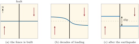
If the fault is locked between earthquakes and each earthquake undoes the slip the plates have accumulated since the last one, the plate motion sets the pace of the cycle.

Proposition 18.2 (Recurrence from the slip rate)

Let a fault segment be loaded at the long-term slip rate $\dot s$, be locked between earthquakes, and slip by the same amount $D$ in each earthquake. Then the recurrence interval of its earthquakes is

$$T = \frac{D}{\dot s} .$$

If only the fraction $c$ of the slip rate is locked, the rest slipping steadily without earthquakes, $T = D/(c\,\dot s)$.

With values typical of the San Andreas fault, a slip of $4\,\mathrm{m}$ in each great earthquake and a slip rate of $20\,\mathrm{mm}\,\mathrm{yr}^{-1}$, the recurrence interval is $200\,\mathrm{yr}$. At Wallace Creek, in central California, a stream channel cut across the fault has been offset by $128\,\mathrm{m}$ in the $3587$ years since it was incised, an average of $36\,\mathrm{mm}\,\mathrm{yr}^{-1}$, close to the rate of about $34\,\mathrm{mm}\,\mathrm{yr}^{-1}$ measured on other offsets there; the last great earthquake on that stretch, in 1857, slipped by nearly $10\,\mathrm{m}$, which at this rate takes about three centuries to accumulate.

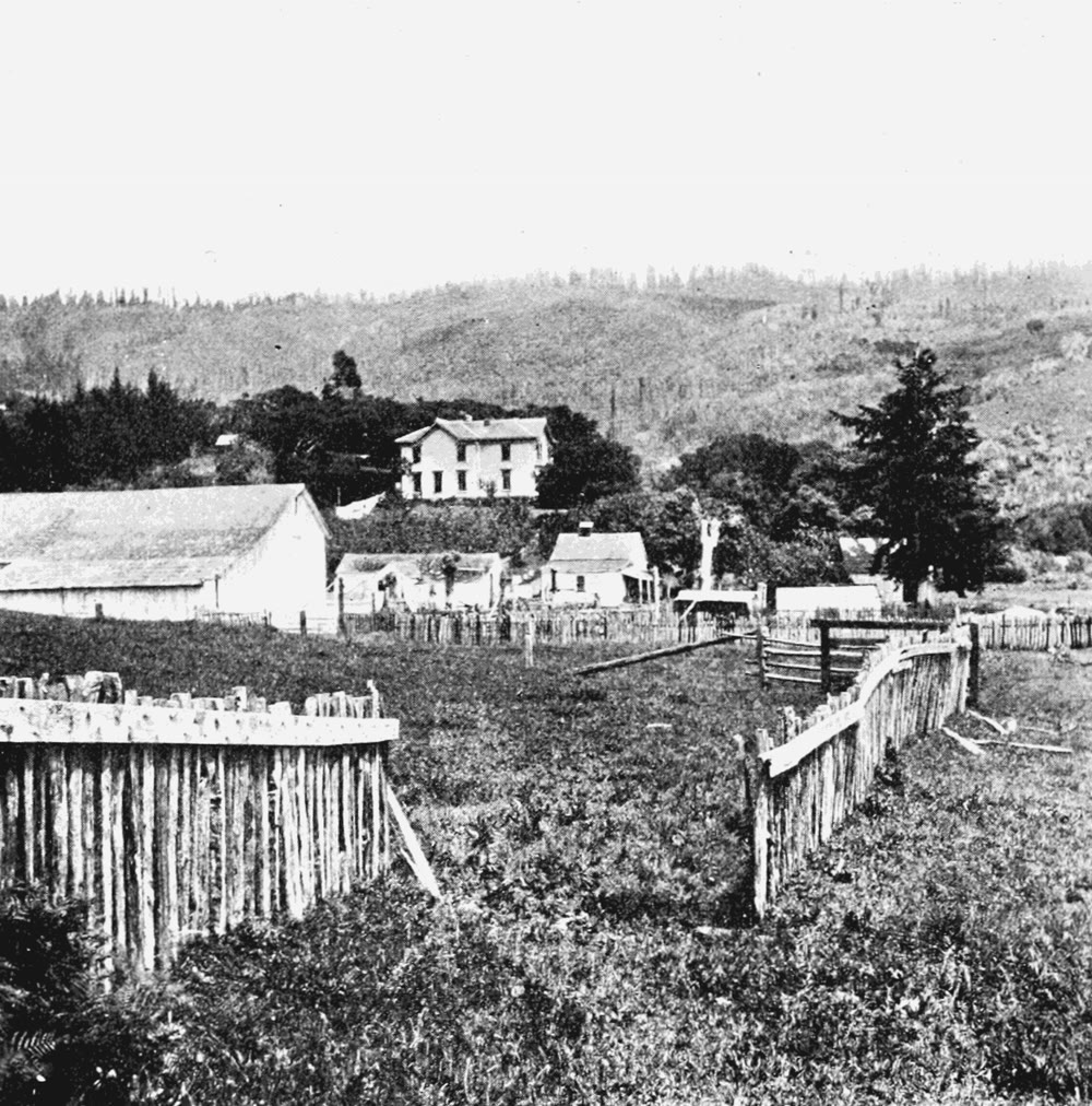
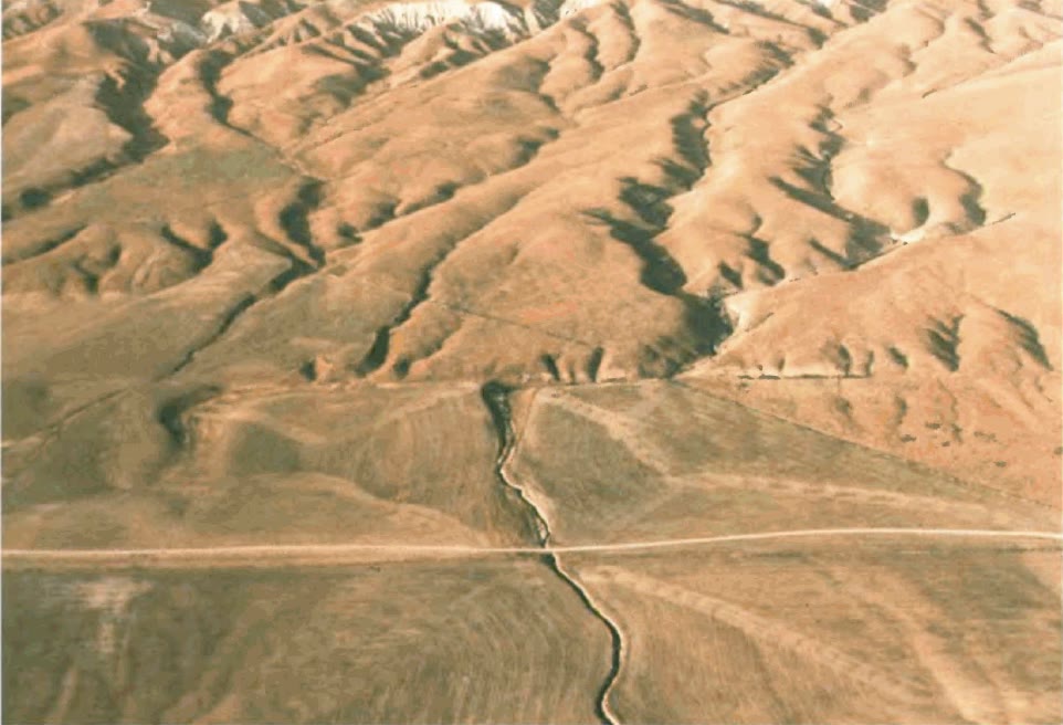
The proposition gives an average, not a timetable. Near Parkfield, on the same fault, an earthquake of magnitude about 6 in 1857 was followed by five more, much alike, on the same stretch of some $30\,\mathrm{km}$, at intervals of nearly 22 years up to 1966; the next was expected before 1993, and came in 2004, with a moment magnitude of 6.0 and without any clear warning sign. The strength of a fault, the slip of each earthquake and the loading by its neighbours all vary from one cycle to the next, and the seismic cycle is better described by a mean recurrence interval and a spread about it than by a period.

Some fault segments do not lock at all. Between Parkfield and San Juan Bautista, the central section of the San Andreas fault creeps: steady slip on the fault takes up nearly all the motion of the plates, and little if any strain builds up on either side, so that this section has no great earthquakes; the great rupture of 1857 started at its southern end and that of 1906 stopped at its northern one. A fault that creeps over part of its area is locked only in part, which is the coefficient $c$ of the proposition.

In the field — Reading past earthquakes in a trench

Instruments have recorded earthquakes for little more than a century, much less than one cycle of most faults. Palaeoseismologists extend the record by reading the ground. A trench a few metres deep is dug across an active fault where layers of sediment have been laid down continuously, in a marsh, a lake or a small alluvial fan. On its walls, each earthquake shows as layers cut and offset by the fault and covered, unbroken, by younger ones; as a scarp buried by later deposits; as sand that liquefied and rose through cracks to spread over the surface of the time. Peat or plant remains in the layers just below and just above each break are dated by radiocarbon, and so bracket the date of each earthquake: one marsh on the San Andreas fault holds the record of twelve. Along coasts, sheets of sand laid down by tsunamis and marshes that sank suddenly by a metre or so, buried under tidal mud, record the great subduction earthquakes. On the San Andreas fault, most of the slip of historical times came with earthquakes of magnitude 6 or more.

History — Harry Fielding Reid and elastic rebound

Harry Fielding Reid, an American physicist, was a member of the state commission that studied the 1906 earthquake. Comparing the positions of points surveyed in 1851–1865, in 1874–1892 and after the earthquake, he found that distant points on the two sides of the San Andreas fault had moved by about $3.2\,\mathrm{m}$ relative to each other since the first survey, a little more than half the slip of about $6\,\mathrm{m}$ on the fault: half a century before the earthquake, the strain that broke the fault was already half built. Only elastic forces could have moved the ground so suddenly, and he called the sudden return elastic rebound. He published it in the second volume of the commission’s report, in 1910; it is still the principal model of the earthquake cycle. Satellite positioning has since measured the bending he could only infer.

18.2 Seismic moment and magnitude

The size of an earthquake is the amount of slip it made, over the area of fault that slipped, weighted by how stiff the rocks are.

Definition 18.3 (Seismic moment)

Let an earthquake slip by the average amount $D$ over a rupture of area $A$, in rocks of shear modulus $\mu$ (the letter also names a coefficient of friction, in Chapter 16; the context tells which). Its seismic moment is

$$M_0 = \mu A D ,$$

in newton metres.

The unit is that of a torque. A slip on a fault sends out the same waves as two pairs of opposed forces, two couples, applied at the focus, and the seismic moment is the moment of each couple (this equivalence, the double couple, is proved in the Year 3 volume). The moment has the dimensions of an energy, but it is not one: the energy radiated as waves is a small fraction of it. For the rocks of the crust, $\mu$ is taken as $30\,\mathrm{GPa}$.

The moment is computed today from the long-period waves recorded around the world. For the Tohoku earthquake of 11 March 2011, the preferred solution of the U.S. Geological Survey gives $M_0 = 5.59 \times 10^{22}\,\mathrm{N}\,\mathrm{m}$. The fault slipped over an area about $400\,\mathrm{km}$ long and $150\,\mathrm{km}$ wide; the definition then gives the average slip

and models of the rupture find up to $50\text{ to }60\,\mathrm{m}$ in its most displaced part.

The magnitude of Book 1 was worked out from the amplitude of the waves on a seismogram. Such magnitudes measure the waves of one period; once a rupture is much longer than their wavelength, a few to some fifty kilometres, the amplitude stops growing with its size, and the magnitude saturates. The body-wave magnitude saturates near 6.5, the surface-wave magnitude near 8.3. In 2011, the first tsunami warning for Tohoku was based on a magnitude of this kind, which falls short for earthquakes of magnitude 8 or more, and it underestimated the waves. The moment does not saturate, and the magnitude is now defined from it.

Definition 18.4 (Moment magnitude)

The moment magnitude of an earthquake of seismic moment $M_0$, in newton metres, is

$$M_w = \tfrac23\left(\log_{10} M_0 - 9.1\right) .$$

Thomas Hanks and Hiroo Kanamori defined the scale in 1979, with the constant 9.05 in place of 9.1, a difference of 0.03 in $M_w$; the constants were chosen to match the older magnitudes where those do not saturate. The magnitude of Book 1 is, for large earthquakes, this number: for Tohoku, $M_w = \tfrac23(\log_{10}5.59 \times 10^{22} - 9.1) = \tfrac23(22.75 - 9.1) = 9.1$; the great Chilean earthquake of 1960 and the Alaskan earthquake of 1964 have moment magnitudes of 9.5 and 9.2, sizes that the older magnitudes could not show.

Proposition 18.5 (One unit of magnitude)

The seismic moment is $M_0 = 10^{1.5 M_w + 9.1}$ newton metres. One unit of moment magnitude multiplies it by $10^{1.5} \approx 31.6$, two units by $1000$. If the energy radiated is a fixed fraction of the moment, it grows in the same ratio.

Kanamori’s approximation, $E_s \approx M_0/(2\times10^4)$ (admitted), is the assumption of the last sentence; the factor of about 32 in energy per unit of magnitude, met in Book 1, is this proposition. Since $M_0 = \mu A D$ and the slip of an earthquake grows with the size of its rupture, a large magnitude needs a large fault. The 1906 rupture, about $430\,\mathrm{km}$ long, broke the seismogenic layer to about $15\,\mathrm{km}$ with an average slip of a few metres: with $D = 4\,\mathrm{m}$, $M_0 = 3 \times 10^{10}\times4.3 \times 10^{5}\times1.5 \times 10^{4} \times 4 = 7.7 \times 10^{20}\,\mathrm{N}\,\mathrm{m}$ and $M_w = 7.9$, the magnitude of the catalogue. A magnitude of 9 needs a rupture of hundreds of kilometres in length and more than a hundred in width, which only the gently dipping interfaces of subduction zones offer.

18.3 Focal mechanisms

The P wave is the first to reach a seismometer. Its first motion, the first swing of the vertical record, is up where the wave arrives as a push, the ground compressed and thrown away from the source, and down where it arrives as a pull. Around an earthquake, pushes and pulls are arranged in a pattern that gives the orientation of the fault and the direction of slip.

Proposition 18.6 (The sign of the first motion)

Let a fault of upward normal $\mathbf n$ slip by the unit vector $\mathbf d$ (the slip of the hanging wall relative to the footwall). The P wave that leaves the focus in the unit direction $\mathbf x$ arrives as a push if $(\mathbf n\cdot\mathbf x)(\mathbf d\cdot\mathbf x) > 0$ and as a pull if $(\mathbf n\cdot\mathbf x)(\mathbf d\cdot\mathbf x) < 0$. The pushes and the pulls thus fill four quadrants, separated by the fault plane ($\mathbf n\cdot\mathbf x = 0$) and by the plane perpendicular to the slip ($\mathbf d\cdot\mathbf x = 0$).

The argument gives the sign only. The amplitude of the first motion, which is proportional to $2(\mathbf n\cdot\mathbf x)(\mathbf d\cdot\mathbf x)$ and so largest at $45{}^{\circ}$ from both planes and zero on them, is admitted here (Year 3 volume).

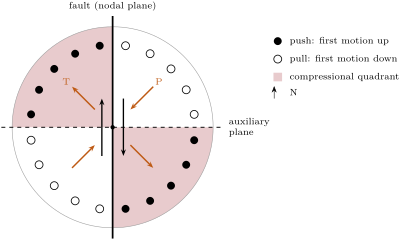
The product $(\mathbf n\cdot\mathbf x)(\mathbf d\cdot\mathbf x)$ does not change when $\mathbf n$ and $\mathbf d$ are exchanged. This symmetry is the central fact of focal mechanisms.

Definition 18.7 (Focal mechanism, nodal plane, auxiliary plane, P axis, T axis)

The first motion of a P wave at a seismometer is the direction, up or down, of the first movement of the ground on the vertical record. The focal mechanism of an earthquake is the orientation of the fault plane and the direction of slip on it, as found from its seismic waves. The two perpendicular planes through the focus that separate the pushes from the pulls are its nodal planes; one is the fault plane, and the other, perpendicular to the slip, is the auxiliary plane. The P axis and the T axis are the directions at $45{}^{\circ}$ from both nodal planes in the middle of the pull quadrants and of the push quadrants:

$$\mathbf P = \frac{\mathbf n - \mathbf d}{\sqrt2}, \qquad \mathbf T = \frac{\mathbf n + \mathbf d}{\sqrt2} .$$

Proposition 18.8 (The two nodal planes)

A slip $\mathbf d$ on the plane of normal $\mathbf n$ and a slip $\mathbf n$ on the plane of normal $\mathbf d$ give the same first motions in every direction. The first motions therefore determine the two nodal planes, the P and T axes and the sense of slip on each plane, but they do not tell which nodal plane is the fault.

To decide which nodal plane slipped, seismologists use other evidence: the plane along which the aftershocks line up, the fault seen at the surface, the plate boundary on which the earthquake lies. For the great Sumatra–Andaman earthquake of 2004, the two nodal planes dip $8{}^{\circ}$ to the north-east and $83{}^{\circ}$ to the south-west. The earlier earthquakes of the region and the plate models both place the sinking slab along a plane dipping gently to the north-east, and the shallow plane is taken as the fault: the earthquake broke the plate interface of the subduction zone, and its aftershocks spread over more than $1300\,\mathrm{km}$.

Because the P axis lies in the middle of the pulls and the T axis in the middle of the pushes, they are often read as the directions of greatest and least compressive stress, $\sigma_1$ and $\sigma_3$. They are only approximations of them. A new fault forms at $45{}^{\circ} - \phi/2$ from $\sigma_1$, not at $45{}^{\circ}$ (Chapter 16), and an old fault may slip at a still different angle, so that the axes of one earthquake can lie tens of degrees from the principal stresses; the stresses of a region are found from the mechanisms of many earthquakes together.

A focal mechanism lives on a sphere around the focus. It is drawn on the lower half of that sphere, which every ray to a distant station crosses, projected onto a disc: a ray of unit vector $\mathbf x = (E, N, U)$, with $U \le 0$, is plotted at

the vertical at the centre and the horizontal on the unit circle. This projection keeps areas (admitted; the projections of the sphere are studied in the Year 3 volume), so that each quadrant covers its true share of the disc. The push quadrants are shaded; the picture is called a beach ball.

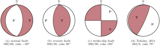
Seismologists give a mechanism by the strike, dip and rake of each nodal plane; the strike is the dip direction minus $90{}^{\circ}$, as in Chapter 17. For Tohoku, the planes are $192/8/78$ and $24/81/91$ in strike, dip and rake, and the P and T axes trend $113$ and $296$ and plunge $36{}^{\circ}$ and $53{}^{\circ}$. The auxiliary plane follows from the fault plane: its normal is $\mathbf d$ and its slip is $\mathbf n$, so that it is found by computing $\mathbf n$ and $\mathbf d$ from the strike, dip and rake, exchanging them, and reading the strike, dip and rake back (exercise 18.7).

Method 18.9 (Reading a beach ball)

1. Look at the centre, which is the vertical. Shaded (a push straight down): a reverse or thrust component; white: a normal component. Two straight diameters crossing at the centre: a strike-slip mechanism.
2. Find the two nodal planes, the curves that bound the quadrants. A plane through the centre is vertical; a plane dips toward the side of the centre on which its curve lies, the more gently the closer the curve is to the rim.
3. Find the T axis in the middle of the shaded quadrants and the P axis in the middle of the white ones: the ground was shortened along P and lengthened along T.
4. For each nodal plane, read or compute the rake, and name the fault it would be with Definition 17.3. The two planes always share the dip-slip sense, normal or reverse, and have opposite strike-slip senses: a strike-slip mechanism gives one dextral and one sinistral plane.
5. Choose the fault plane from the aftershocks, the geology or the plate boundary.

In the lab — At a seismological observatory

Within minutes of a large earthquake, its waves have been recorded by hundreds of stations, and the data reach the analysts of the observatories in near real time. The first arrivals of the P wave, which reach the stations later the farther they are, are picked on the records to locate the focus. Then the long, slow waves recorded over the next tens of minutes are compared with waves computed for trial sources; the source whose waves fit best gives the moment tensor, which contains the seismic moment, the moment magnitude and the two nodal planes together. For small earthquakes, too weak for this, the analysts read the first motions on the nearest records and fit the nodal planes to them, the way described in this section. Each solution is published with its uncertainties, and revised as more data arrive.

18.4 Measuring the loading: geodesy

Between earthquakes, a locked fault is invisible to seismometers, but the ground around it moves. Permanent satellite-positioning stations measure that motion, and the way their velocities change across a fault tells how deep it is locked.

Definition 18.10 (Locking depth)

The locking depth of a fault is the depth down to which it is locked between earthquakes, the fault below sliding steadily at the long-term rate; it is the depth of the part of the fault that slips in the next earthquake.

Proposition 18.11 (Interseismic velocity across a strike-slip fault)

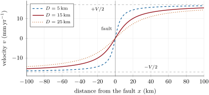
Let a vertical strike-slip fault in an elastic half-space be locked from the surface to the depth $D$, and slide at the rate $V$ below it. The velocity of the surface parallel to the fault, at the distance $x$ from it, is

$$v(x) = \frac{V}{\pi}\arctan\frac{x}{D} .$$

If the fault then slips by $s$ from the surface to the depth $D$ in an earthquake, the surface moves by $u(x) = (s/\pi)\arctan(D/x)$ for $x > 0$, and by $-u(-x)$ for $x < 0$.

This model, due to Savage and Burford, is the simplest form of the elastic rebound, and the curve of the fence of the first figure. Its properties follow from the formula.

Proposition 18.12 (Reading the interseismic profile)

In the model of Proposition 18.11:

1. far from the fault the velocity tends to $\pm V/2$, the two plates moving at $V$ relative to each other;
2. half of the change of velocity across the fault happens within the distance $D$ of it: $v(\pm D) = \pm V/4$;
3. the shear-strain rate of the surface, $\mathrm dv/\mathrm dx$, is largest on the fault, where it equals $V/(\pi D)$;
4. if the fault, after loading for the time $t$, slips by $s = Vt$ in an earthquake, the ground ends up displaced by $\pm s/2$ everywhere on either side: the cycle leaves no permanent bending, only the offset $s$ on the fault.

Property (b) gives the locking depth from a profile of stations: it is the distance from the fault at which the velocity has changed by a quarter of $V$ from its value on the fault. A shallow lock concentrates the strain near the fault (the figure below), a deep one spreads it over a wide belt. Along the San Andreas system, the locking depths found from geodesy range from nearly 0, on creeping segments, to $26\,\mathrm{km}$, and agree with the depths of the earthquakes: the locked part is the seismogenic layer of Chapter 16. For a slip rate of $34\,\mathrm{mm}\,\mathrm{yr}^{-1}$ and a locking depth of $15\,\mathrm{km}$, the shear-strain rate on the fault is $0.034/(\pi\times15\,000) = 7.2 \times 10^{-7}$ per year, which bends a line across the fault by less than a millimetre per kilometre in a year, yet stores, over two centuries, the several metres of slip of a great earthquake.

Satellite positioning measures the ground at a few stations. Radar satellites measure it everywhere: two radar images of the same area taken from the same orbit at different times are compared wave by wave, and the difference of phase maps the change of the distance between the ground and the satellite, point by point, a hundred metres apart, with no network of stations set up in advance. The first such map, of a large Californian earthquake in 1992, showed its coseismic displacement in a single picture and agreed with the slip measured in the field and by surveying; the technique, radar interferometry, belongs to the Year 3 volume.

18.5 How often: the Gutenberg–Richter law

Small earthquakes are far more common than large ones, and in a remarkably regular way.

Proposition 18.13 (Gutenberg–Richter law)

In a region and a period, the number $N$ of earthquakes of magnitude at least $M$ follows

$$\log_{10} N = a - bM ,$$

for every $M$ above the magnitude of completeness of the catalogue, with constants $a$ and $b$ that depend on the region; $b$ is close to 1 in most active regions.

The law is a result of observation, published by Beno Gutenberg and Charles Richter for California in 1944 and since found everywhere; no theory yet derives it, nor the value of $b$.

Definition 18.14 (b-value, magnitude of completeness)

The constant $b$ of the Gutenberg–Richter law of a region is its b-value. The magnitude of completeness of a catalogue is the smallest magnitude above which it records every earthquake of the region and period.

A b-value of 1 means ten times fewer earthquakes for each unit of magnitude. Below the magnitude of completeness, the counts fall short of the line, because small earthquakes are recorded by too few stations to be located: the law seems to bend, and $b$ must be measured above it. For the whole Earth, divided into shallow, intermediate and deep earthquakes, the measured values lie between 0.72 and 1.34, but they differ by $30\,\%$ or more from one catalogue, range of magnitude or method to another: a value far from 1 is first a reason to check the catalogue.

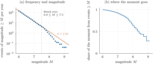
For the world catalogue of the figure, the law with $a = 8.20$ and $b = 1.01$ predicts 14 earthquakes of magnitude 7 or more a year, as observed, and 1.35 of magnitude 8 or more, while 40 in fifty years, 0.8 a year, were recorded. Whether the largest earthquakes are truly fewer than the line, as the finite size of faults would suggest, or only rare enough to be missing from fifty years, is not settled by so few events. About one magnitude in nine in this catalogue is a surface-wave or body-wave magnitude, which saturate; the largest events all have moment magnitudes.

The many small earthquakes do little of the work. Their number grows ten times for each unit of magnitude less, but their moments shrink 31.6 times.

Proposition 18.15 (The largest earthquakes release most of the moment)

Let earthquakes follow the Gutenberg–Richter law with $b < 1.5$, up to a largest magnitude $M_{\max}$, and let them be grouped in bins one unit of magnitude wide, the top bin ending at $M_{\max}$. Then the earthquakes of the top bin release more than the fraction $1 - 10^{-(1.5 - b)}$ of the total moment, however small the smallest magnitude counted: more than $68\,\%$ for $b = 1$.

In the world catalogue the share is of this order: the top unit of magnitude, from 8.1 to 9.1, released over half of the moment of fifty years, and the two largest earthquakes, Sumatra–Andaman in 2004 and Tohoku in 2011, with magnitudes of 9.1, released $29\,\%$ of it by themselves. The moment a plate boundary must release is set by its slip rate; the proposition says that it is released almost entirely in its largest earthquakes, and that the many small ones, however frequent, do not relieve a fault of the next great one.

18.6 Exercises

Exercise 18.1 ★

(a) Compute the moment magnitude of an earthquake of seismic moment $4 \times 10^{17}\,\mathrm{N}\,\mathrm{m}$. (b) The Tohoku earthquake had $M_0 = 5.59 \times 10^{22}\,\mathrm{N}\,\mathrm{m}$: check its magnitude. (c) What seismic moment has an earthquake of magnitude 7.0?

Solution

Solution of Exercise 18.1.

(a) $\log_{10}(4 \times 10^{17}) = 17.60$, so $M_w = \tfrac23(17.60 - 9.1) = 5.67$. (b) $\log_{10}(5.59 \times 10^{22}) = 22.75$ and $M_w = \tfrac23(22.75 - 9.1) = 9.10$. (c) $M_0 = 10^{1.5\times7.0 + 9.1} = 10^{19.6} = 3.98 \times 10^{19}\,\mathrm{N}\,\mathrm{m}$.

Exercise 18.2 ★

A strike-slip fault is loaded at $25\,\mathrm{mm}\,\mathrm{yr}^{-1}$, and its earthquakes each slip by about $3\,\mathrm{m}$. (a) What is their recurrence interval if the fault is fully locked between them? (b) And if half the slip rate is taken up by steady creep?

Solution

Solution of Exercise 18.2.

(a) $T = D/\dot s = 3\,\mathrm{m}/0.025\,\mathrm{m}\,\mathrm{yr}^{-1} = 120\,\mathrm{yr}$. (b) With $c = 0.5$, $T = D/(c\dot s) = 240\,\mathrm{yr}$: the creep takes up half the motion, and the earthquakes, of the same slip, come half as often.

Exercise 18.3 ★

How many times larger is the seismic moment of an earthquake of magnitude 7.4 than that of an earthquake of magnitude 6.2? How many earthquakes of magnitude 6.2 would release the same moment?

Solution

Solution of Exercise 18.3.

By Proposition 18.5, the ratio of the moments is $10^{1.5\times(7.4 - 6.2)} = 10^{1.8} = 63.1$: it takes 63 earthquakes of magnitude 6.2 to release the moment of one of magnitude 7.4.

Exercise 18.4 ★

In a region with $b = 1$, a thousand earthquakes of magnitude 3 or more are recorded each year. How many of magnitude 5 or more, and of magnitude 6 or more, are expected each year? What is the mean time between earthquakes of magnitude 7 or more?

Solution

Solution of Exercise 18.4.

With $b = 1$, each unit of magnitude divides the count by 10: 10 earthquakes of magnitude 5 or more a year, 1 of magnitude 6 or more, and 0.1 of magnitude 7 or more, that is one every 10 years on average.

Exercise 18.5 ★★

The 1906 earthquake broke the San Andreas fault over about $430\,\mathrm{km}$. (a) Assuming the rupture reached $15\,\mathrm{km}$ deep with an average slip of $4\,\mathrm{m}$, and $\mu = 30\,\mathrm{GPa}$, compute its seismic moment and moment magnitude. (b) How much does the magnitude change if the rupture was only $10\,\mathrm{km}$ deep? (c) Which of the two estimates is closer to 7.9?

Solution

Solution of Exercise 18.5.

(a) $A = 4.3 \times 10^{5} \times 1.5 \times 10^{4}\,\mathrm{m} = 6.45 \times 10^{9}\,\mathrm{m}^{2}$, and $M_0 = 3 \times 10^{10}\times6.45 \times 10^{9}\times4 = 7.74 \times 10^{20}\,\mathrm{N}\,\mathrm{m}$; $\log_{10}M_0 = 20.89$ and $M_w = \tfrac23(20.89 - 9.1) = 7.86$. (b) A depth of $10\,\mathrm{km}$ divides the area and the moment by 1.5, which lowers the magnitude by $\tfrac23\log_{10}1.5 = 0.12$, to 7.74. (c) The first, 7.86, rounds to the 7.9 of the catalogue; the second is a little low. The magnitude is not very sensitive to the depth: a factor of 1.5 on the area is only 0.12 of magnitude.

Exercise 18.6 ★★

The rupture of the Tohoku earthquake was about $400\,\mathrm{km}$ long and $150\,\mathrm{km}$ wide, and its moment $5.59 \times 10^{22}\,\mathrm{N}\,\mathrm{m}$. (a) Compute its average slip with $\mu = 30\,\mathrm{GPa}$. (b) The Pacific plate sinks beneath Japan at about $83\,\mathrm{mm}\,\mathrm{yr}^{-1}$: how long does it take to accumulate this slip if the interface is fully locked? (c) And if the locked fraction is 0.8, or 0.5?

Solution

Solution of Exercise 18.6.

(a) $D = M_0/(\mu A) = 5.59 \times 10^{22}/(3 \times 10^{10}\times4 \times 10^{5}\times1.5 \times 10^{5}) = 31.1\,\mathrm{m}$. (b) $31.1\,\mathrm{m}/0.083\,\mathrm{m}\,\mathrm{yr}^{-1} = 374\,\mathrm{yr}$. (c) With the locked fraction 0.8, $31.1/(0.8\times0.083) = 468\,\mathrm{yr}$; with 0.5, $749\,\mathrm{yr}$. The less the interface is locked, the longer the slip of one great earthquake takes to build up; the average slip found here with a rectangle of $400\,\mathrm{km} \times 150\,\mathrm{km}$ and $\mu = 30\,\mathrm{GPa}$ is itself only an estimate, and the real slip was far from uniform.

Exercise 18.7 ★★

One nodal plane of the 2004 Sumatra–Andaman earthquake has strike $329$, dip $8{}^{\circ}$ and rake $110{}^{\circ}$. (a) Write $\mathbf n$ and $\mathbf d$ in east, north and up components. (b) Find the strike, dip and rake of the auxiliary plane. (c) Find the trends and plunges of the P and T axes. (d) Which plane is the fault, and what kind of fault is it?

Solution

Solution of Exercise 18.7.

(a) The strike is $\phi = 329$, the dip direction $a = 059$, the dip $\delta = 8{}^{\circ}$. Then $\mathbf s = (\sin329, \cos329, 0) = (-0.5150, 0.8572, 0)$, $\mathbf u = (-\cos8\sin59, -\cos8\cos59, \sin8) = (-0.8488, -0.5100, 0.1392)$, $\mathbf n = (\sin8\sin59, \sin8\cos59, \cos8) = (0.1193, 0.0717, 0.9903)$, and with $r = 110{}^{\circ}$,

$$\mathbf d = \cos110\,\mathbf s + \sin110\,\mathbf u = (-0.6215, -0.7724, 0.1308) .$$

(b) The auxiliary plane has the normal $\mathbf d$ and the slip $\mathbf n$. Taking the normal upward, it dips $\arccos 0.1308 = 82.5{}^{\circ}$ toward $\arctan(-0.6215/-0.7724) = 218.8$, so its strike is $128.8$; the slip $\mathbf n$ projected on its strike and up-dip vectors gives the rake $87.2{}^{\circ}$. Rounded: $129/83/87$, the second plane of the published solution. (c) $\mathbf P = (\mathbf n - \mathbf d)/\sqrt2$ trends $221$ and plunges $37{}^{\circ}$; $\mathbf T = (\mathbf n + \mathbf d)/\sqrt2$ trends $036$ and plunges $52{}^{\circ}$ (published: $222/38$ and $36/52$). (d) The shallow plane, dipping $8{}^{\circ}$ toward $059$, along the subducting slab: a reverse fault with a rake of $110{}^{\circ}$, and, dipping less than $45{}^{\circ}$, a thrust, the plate interface of the subduction zone.

Exercise 18.8 ★★

A vertical fault striking $045$ slips dextrally. (a) For waves leaving the focus horizontally toward stations due north, east, south and west, which arrive as pushes and which as pulls? (b) Give the trends of the P and T axes. (c) Show that a sinistral slip on a vertical plane striking $135$ gives the same first motions.

Solution

Solution of Exercise 18.8.

(a) The plane dips toward $135$, so $\mathbf n = (\sin135, \cos135, 0) = (0.707, -0.707, 0)$; a dextral slip has $r = 180{}^{\circ}$, $\mathbf d = -\mathbf s = (-0.707, -0.707, 0)$. Toward the north, $\mathbf x = (0, 1, 0)$: $(\mathbf n\cdot\mathbf x)(\mathbf d\cdot\mathbf x) = (-0.707)(-0.707) > 0$, a push. East: $(0.707)(-0.707) < 0$, a pull. South: a push; west: a pull. (b) $\mathbf P = (\mathbf n - \mathbf d)/\sqrt2 = (1, 0, 0)$: the P axis is horizontal and trends $090$–$270$; $\mathbf T = (0, -1, 0)$ trends $000$–$180$. (c) The vertical plane striking $135$–$315$ has the normal $\mathbf d$. With the slip $\mathbf n$, the block on its south-west side, into which $\mathbf d$ points, moves toward $135$; seen from the north-east block, looking south-west, that is to the left: a sinistral slip. By Proposition 18.8, this slip gives the same first motions in every direction.

Exercise 18.9 ★★

Across a locked strike-slip fault, the far-field stations on the two sides move at $40\,\mathrm{mm}\,\mathrm{yr}^{-1}$ relative to each other. A station $10\,\mathrm{km}$ from the fault moves at $10\,\mathrm{mm}\,\mathrm{yr}^{-1}$ relative to the fault trace. (a) Find the locking depth. (b) Predict the velocity of a station $30\,\mathrm{km}$ from the fault. (c) Compute the shear-strain rate on the fault.

Solution

Solution of Exercise 18.9.

(a) $V = 40\,\mathrm{mm}\,\mathrm{yr}^{-1}$ and $v = V/4$ at $10\,\mathrm{km}$, so by Proposition 18.12(b) $D = 10\,\mathrm{km}$; directly, $D = x/\tan(\pi v/V) = 10/\tan(\pi/4) = 10\,\mathrm{km}$. (b) $v(30) = (40/\pi)\arctan 3 = 15.9\,\mathrm{mm}\,\mathrm{yr}^{-1}$. (c) $V/(\pi D) = 0.040/(\pi\times10\,000) = 1.27 \times 10^{-6}$ per year.

Exercise 18.10 ★★★

(a) Show that, if $b$ were larger than 1.5, the total moment of the earthquakes of a region would be dominated by the smallest ones. (b) What share of the moment does the top unit of magnitude release at least, for $b = 0.8$? (c) With the world catalogue’s $a = 8.20$ and $b = 1.01$ per year, how many earthquakes of magnitude 9 or more would the law predict in fifty years? The catalogue of 1976–2025 holds two; comment.

Solution

Solution of Exercise 18.10.

(a) The moments of the bins are still $C q^k$ with $q = 10^{1.5 - b}$, but now $q < 1$: the moment of the bins decreases toward the large magnitudes, and the bottom bin, $k = 0$, carries the share $C/S = (1 - q)/(1 - q^{K+1}) > 1 - q$, the mirror image of Proposition 18.15. The smallest earthquakes counted would then dominate, and the total would grow without limit as smaller and smaller ones were included. (b) $1 - 10^{-0.7} = 0.80$: at least $80\,\%$. (c) $\log_{10}N = 8.20 - 1.01\times9 = -0.89$, so $N = 0.13$ a year and about 6.4 in fifty years, three times the two observed. The line, fitted between magnitudes 6 and 7.5, overestimates the largest earthquakes; either the law bends down at the top, as the finite size of faults suggests, or fifty years are too few to sample events that come once in decades. Both are possible with two events.

Exercise 18.11 ★★★

A straight fence is built across a locked dextral fault with $V = 34\,\mathrm{mm}\,\mathrm{yr}^{-1}$ and $D = 15\,\mathrm{km}$. (a) After 150 years, by how much have the posts $1\,\mathrm{km}$, $15\,\mathrm{km}$ and $50\,\mathrm{km}$ east of the fault moved along it, relative to the post on the fault? (b) The fault then slips by the whole deficit in an earthquake. What is the slip, and how far does each of the three posts move during the earthquake? (c) Check part (d) of Proposition 18.12 on the three posts.

Solution

Solution of Exercise 18.11.

(a) In 150 years a post at $x$ moves by $150\,v(x) = 150\times(34/\pi) \arctan(x/15)$ millimetres relative to the post on the fault: $0.11\,\mathrm{m}$ at $1\,\mathrm{km}$, $1.28\,\mathrm{m}$ at $15\,\mathrm{km}$, $2.08\,\mathrm{m}$ at $50\,\mathrm{km}$, toward the south for a dextral fault seen from the west. (b) The slip deficit is $s = 0.034\,\mathrm{m}\,\mathrm{yr}^{-1}\times150\,\mathrm{yr} = 5.1\,\mathrm{m}$. During the earthquake the posts move by $(s/\pi)\arctan(D/x)$: $2.44\,\mathrm{m}$ at $1\,\mathrm{km}$, $1.28\,\mathrm{m}$ at $15\,\mathrm{km}$, $0.47\,\mathrm{m}$ at $50\,\mathrm{km}$. (c) The sums are $0.11 + 2.44$, $1.28 + 1.28$ and $2.08 + 0.47$, all $2.55\,\mathrm{m}$ $= s/2$: after the earthquake the fence is straight again on the east side, displaced by $s/2$, and the west side, by symmetry, by $-s/2$.

Exercise 18.12 ★★★

An earthquake has a horizontal P axis trending $000$ and a horizontal T axis trending $090$. (a) Show that its nodal planes are vertical and strike $045$ and $135$, using $\mathbf n$, $\mathbf d = (\mathbf T \pm \mathbf P)/\sqrt2$. (b) Give the sense of slip on each plane. (c) If the fault had formed as a new fault in a rock with $\phi = 30{}^{\circ}$, under a $\sigma_1$ along the P axis, at what strikes would it lie, and why is the P axis only an approximation of $\sigma_1$? (d) A mapped fault nearby strikes $040$. Which nodal plane is likely the fault, and what is its sense of slip?

Solution

Solution of Exercise 18.12.

(a) $\mathbf P = (0, 1, 0)$ and $\mathbf T = (1, 0, 0)$. The pair $\mathbf n = (\mathbf T + \mathbf P)/\sqrt2 = (0.707, 0.707, 0)$, $\mathbf d = (\mathbf T - \mathbf P)/\sqrt2 = (0.707, -0.707, 0)$ satisfies $\mathbf P = (\mathbf n - \mathbf d)/\sqrt2$ and $\mathbf T = (\mathbf n + \mathbf d)/\sqrt2$. Both vectors are horizontal, so both nodal planes are vertical: the plane of normal $\mathbf n$ (toward $045$) strikes $135$–$315$, the plane of normal $\mathbf d$ (toward $135$) strikes $045$–$225$. (b) On the plane striking $315$, the block on the north-east side moves along $\mathbf d$, toward $135$: seen from the other block, to the right, a dextral slip. On the plane striking $045$, the block on the south-east side moves along $\mathbf n$, toward $045$: a sinistral slip. (c) A new fault makes $45{}^{\circ} - \phi/2 = 30{}^{\circ}$ with $\sigma_1$: with $\sigma_1$ trending $000$, the faults would strike $030$ (sinistral) and $330$ (dextral), $15{}^{\circ}$ from the nodal planes. The P axis is fixed at $45{}^{\circ}$ from the nodal planes by geometry, whatever the friction of the rock, so it coincides with $\sigma_1$ only if the fault slipped at $45{}^{\circ}$ from it. (d) The fault striking $040$ is $5{}^{\circ}$ from the nodal plane striking $045$: that plane is likely the fault, and the slip on it is sinistral.

18.7 Problem: The next great earthquake on a locked fault

Problem 18.1

Weekend problem — a locked segment of a strike-slip plate boundary, from its loading and its past earthquakes to the magnitude of the next

A straight, vertical strike-slip fault forms the boundary between two plates. One segment of it, $250\,\mathrm{km}$ long, is locked; its earthquakes start no deeper than $15\,\mathrm{km}$. Trenches dug across it date its last four great earthquakes to about 1050, 1290, 1480 and 1712, with offsets of $7.0$, $6.0$, $5.5$ and $7.5\,\mathrm{m}$. Permanent stations far from the fault on the two sides move at $30\,\mathrm{mm}\,\mathrm{yr}^{-1}$ relative to each other. Take $\mu = 30\,\mathrm{GPa}$, the year 2025 as the present, and give magnitudes to 0.01.

Part I — The loading.

1. Compute the intervals between the four earthquakes and their mean.
2. Compute the mean offset, and the recurrence interval it implies with Proposition 18.2 for a fully locked fault.
3. Compute the slip rate implied by the trench alone, from the offsets of the last three earthquakes and the time between the first and the last. Compare with the geodetic rate.
4. How long ago was the last earthquake, and what slip deficit has accumulated since, if the segment is fully locked?
5. Compare this deficit with the offsets in the trench. Is the next earthquake overdue?
6. Why can the trench not give the date of the next one?

Part II — The size of the next earthquake.

7. What is the area of the locked part of the segment?
8. Compute the seismic moment of an earthquake that would release the whole deficit.
9. Compute the moment magnitude of the 1712 earthquake, assuming it broke the same area with its trench offset as average slip.
10. By what factor does the moment of the next earthquake exceed that of 1712, and how many units of magnitude is that?
11. If only half of the segment broke, with the same slip, what would the magnitude be?
12. Give the seismic moment that the segment accumulates each year.

Part III — Frequency and energy.

13. The regional catalogue follows $\log_{10} N = 4.3 - M$ per year, from all the faults of the region. What is its b-value, and how many earthquakes of magnitude 5 or more, and 6 or more, does it give each year?
14. What mean time between earthquakes of magnitude 7 or more does it give, and of magnitude 8 or more?
15. Compare the recurrence of a great earthquake from the catalogue with the one from the trench. What does the difference say about using the law of small earthquakes to forecast great ones?
16. The earthquakes of magnitude 5 to 8 of the regional law release, all together, about $5.5 \times 10^{17}\,\mathrm{N}\,\mathrm{m}$ a year. What fraction of the moment of the segment is that?
17. How many times more energy than an earthquake of magnitude 6 would the next great earthquake radiate?
18. Using Proposition 18.15, explain why the moderate earthquakes of the segment do not relieve it.

Part IV — The locking depth from the stations.

19. A profile of stations across the segment gives, relative to the fault trace, the velocities $-11.6$, $-7.5$, $-3.1$, $3.1$, $7.5$ and $11.6\,\mathrm{mm}\,\mathrm{yr}^{-1}$ at $x = -40$, $-15$, $-5$, $5$, $15$ and $40\,\mathrm{km}$. Check that the profile is antisymmetric, and give the velocities expected far from the fault.
20. From the station at $15\,\mathrm{km}$, compute the locking depth.
21. Compute it again from the stations at $5\,\mathrm{km}$ and $40\,\mathrm{km}$, and explain the small differences.
22. Compare the locking depth with the depth of the earthquakes, and say why they should agree.
23. Compute the shear-strain rate on the fault.
24. To 0.01, what is the moment magnitude of the earthquake that would release the whole slip deficit of the segment?

Solution

Solution of Problem 18.1.

1. The intervals are $1290 - 1050 = 240$, $1480 - 1290 = 190$ and $1712 - 1480 = 232$ years; their mean is $220.7\,\mathrm{yr}$.

2. The mean offset is $(7.0 + 6.0 + 5.5 + 7.5)/4 = 6.5\,\mathrm{m}$, and $T = 6.5/0.030 = 216.7\,\mathrm{yr}$, close to the mean interval.

3. The offsets of the last three earthquakes, $6.0 + 5.5 + 7.5 = 19.0\,\mathrm{m}$, accumulated between 1050 and 1712, in 662 years: $19.0\,\mathrm{m} /662\,\mathrm{yr} = 28.7\,\mathrm{mm}\,\mathrm{yr}^{-1}$, $4\,\%$ less than the geodetic $30\,\mathrm{mm}\,\mathrm{yr}^{-1}$. The two agree within the uncertainty of the dates and offsets: the segment releases nearly all of its loading in its great earthquakes.

4. $2025 - 1712 = 313$ years, and the deficit is $0.030\,\mathrm{m}\,\mathrm{yr}^{-1}\times313\,\mathrm{yr} = 9.39\,\mathrm{m}$.

5. The deficit exceeds every offset in the trench, the largest being $7.5\,\mathrm{m}$, and the time since 1712 exceeds the longest interval, 240 years. In that sense the segment is overdue; it does not mean that the earthquake is imminent, only that the fault already holds more slip than it has ever released at once in the record.

6. The intervals range from 190 to 240 years and the offsets from $5.5\text{ to }7.5\,\mathrm{m}$: the cycle is not periodic, and the strength of the fault at the next earthquake is unknown. The trench gives a mean and a spread, from which a probability can be estimated, not a date.

7. $A = 250\,\mathrm{km}\times15\,\mathrm{km} = 3750\,\mathrm{km}^{2} = 3.75 \times 10^{9}\,\mathrm{m}^{2}$.

8. $M_0 = 3 \times 10^{10}\times3.75 \times 10^{9}\times9.39 = 1.06 \times 10^{21}\,\mathrm{N}\,\mathrm{m}$.

9. $M_0 = 3 \times 10^{10}\times3.75 \times 10^{9}\times7.5 = 8.44 \times 10^{20}\,\mathrm{N}\,\mathrm{m}$, so $M_w = \tfrac23(20.926 - 9.1) = 7.88$.

10. The ratio is $9.39/7.5 = 1.25$, which is $\tfrac23\log_{10}1.25 = 0.07$ of magnitude.

11. Half the area halves the moment and lowers the magnitude by $\tfrac23\log_{10}2 = 0.20$: $M_w = 7.75$.

12. $\mu A V = 3 \times 10^{10}\times3.75 \times 10^{9}\times0.030 = 3.38 \times 10^{18}\,\mathrm{N}\,\mathrm{m}$ per year.

13. $b = 1$. $N(5) = 10^{4.3 - 5} = 0.20$ a year and $N(6) = 0.020$ a year.

14. $N(7) = 0.0020$ a year: one every 500 years; $N(8) = 0.00020$ a year: one every $5000$ years.

15. The law gives one earthquake of magnitude 7.95 or more every $1/10^{4.3 - 7.95} = 4500$ years, the trench one every 220 years, twenty times more often. The law is fitted to the many small earthquakes of all the faults of the region; extrapolated to the great earthquakes of one segment, it underestimates them badly. The recurrence of great earthquakes on a fault is taken from its own record and from its loading, not from the small ones.

16. $5.5 \times 10^{17}/3.38 \times 10^{18} = 0.16$: the moderate earthquakes release $16\,\%$ of the moment the segment accumulates.

17. By Proposition 18.5, $10^{1.5\times(7.95 - 6)} = 10^{2.92} \approx 840$ times more.

18. With $b = 1$, the moment of the earthquakes is dominated by the largest: whatever the moderate earthquakes do, they release a minor share, here $16\,\%$, and the remaining $84\,\%$, the slip deficit, waits for the great earthquake.

19. $v(-x) = -v(x)$ for each pair, so the profile is antisymmetric. Far from the fault the velocities tend to $\pm V/2 = \pm15\,\mathrm{mm}\,\mathrm{yr}^{-1}$.

20. $D = x/\tan(\pi v/V) = 15/\tan(\pi\times7.5/30) = 15/\tan45{}^{\circ} = 15\,\mathrm{km}$: at the locking depth the velocity is $V/4$.

21. At $5\,\mathrm{km}$: $D = 5/\tan(\pi\times3.1/30) = 5/\tan18.6{}^{\circ} = 14.9\,\mathrm{km}$; at $40\,\mathrm{km}$: $D = 40/\tan69.6{}^{\circ} = 14.9\,\mathrm{km}$. The velocities are given to $0.1\,\mathrm{mm}\,\mathrm{yr}^{-1}$, and that rounding alone moves $D$ by about $0.1\,\mathrm{km}$; with real data, the noise of each station would be larger, and the locking depth would be fitted to all the stations at once.

22. The locking depth, $15\,\mathrm{km}$, equals the depth of the deepest earthquakes. The locked part of the fault is its brittle part, the seismogenic layer, where friction holds it between earthquakes and fails in them; below, the warmer rock creeps (Chapter 16) and the fault slides steadily, which is the slip at the rate $V$ below $D$ of the model.

23. $V/(\pi D) = 0.030/(\pi\times15\,000) = 6.4 \times 10^{-7}$ per year.

24. With $M_0 = 1.056 \times 10^{21}\,\mathrm{N}\,\mathrm{m}$, $\log_{10}M_0 = 21.024$ and $M_w = \tfrac23(21.024 - 9.1) = 7.949$. To 0.01, the earthquake that would release the whole deficit of the segment has the moment magnitude 7.95.