29The Circulation of the Ocean

In 1992, during a storm in the North Pacific, a container washed overboard from a ship sailing from Hong Kong to the United States. It broke open and released about $29\,000$ rubber ducks and other bath toys, which floated away and travelled far and wide; the places where some of them were later found helped scientists to understand the currents that had carried them. Floating toys follow the surface water, and the surface water of the oceans does not wander at random: it turns in basin-wide gyres, races north in narrow currents along the western coasts of the oceans, and rises or sinks in a few chosen places. This chapter explains how the wind sets the upper ocean moving, why the water moves at right angles to the wind that pushes it, why the strongest currents hug the western sides of the oceans, and how a slow overturning carries water to the abyss and back.

You already know

The physics volumes give the Coriolis force. Chapter 28 wrote its horizontal part as $-f\,\vec k\times\vec v$, with the Coriolis parameter $f = 2\Omega\sin\varphi$ ($\Omega = 7.292 \times 10^{-5}\,\mathrm{rad}\,\mathrm{s}^{-1}$), and found the trade winds, easterlies between the equator and about $30{}^{\circ}$, and the westerlies beyond; it also defined the mean meridional streamfunction of an overturning. Chapter 26 gave the mixed layer and the thermocline, the density of seawater, the T–S diagram and the water masses of the South Atlantic, and Chapter 27 the poleward heat transport shared by the atmosphere and the ocean. Book 1 described the surface currents and the great gyres; Book 2 the upwelling of cold water along some coasts.

29.1 The wind and the surface currents

The wind moves the sea by rubbing on it. Its force is spread over the surface, and it is measured, like a pressure, per unit area.

Definition 29.1 (Wind stress)

The wind stress $\vec T$ is the horizontal force per unit area exerted by the wind on the sea surface, in pascals. It is the downward transfer of the horizontal momentum of the air into the ocean, and points nearly along the wind. Its size is given by the bulk formula

$$T = \rho_a C_D U_{10}^2,$$

where $\rho_a = 1.3\,\mathrm{kg}\,\mathrm{m}^{-3}$ is the density of air, $U_{10}$ the wind speed $10\,\mathrm{m}$ above the sea and $C_D$ a dimensionless drag coefficient.

The drag coefficient is measured with fast instruments that record the turbulent fluctuations of the wind a few metres above the waves. For a neutrally stable air, the measurements of Yelland and Taylor give

with $U_{10}$ in metres per second. A wind of $10\,\mathrm{m}/\mathrm{s}$ has $C_D = 1.31 \times 10^{-3}$ and exerts $T = 1.3 \times 1.31 \times 10^{-3} \times 100 = 0.170\,\mathrm{Pa}$; a wind of $5\,\mathrm{m}/\mathrm{s}$, $0.040\,\mathrm{Pa}$; a gale of $20\,\mathrm{m}/\mathrm{s}$, $1.05\,\mathrm{Pa}$. Doubling the wind from 10 to $20\,\mathrm{m}/\mathrm{s}$ multiplies the stress by $6.2$, not by $4$: rougher seas grip the wind harder. These stresses are minute, a millionth of the atmospheric pressure, but they act without pause on the whole ocean.

The pattern of the stress follows that of the winds. Between the trade winds of the tropics, blowing towards the west, and the westerlies of the mid-latitudes, blowing towards the east, the surface water of each ocean basin is set turning.

Definition 29.2 (Gyre; subtropical and subpolar gyres)

A gyre is a large system of rotating ocean currents filling an ocean basin. A subtropical gyre lies between the trade winds and the westerlies and turns clockwise in the Northern Hemisphere and anticlockwise in the Southern. A subpolar gyre lies on the poleward side of the westerlies and turns the other way.

There are five subtropical gyres, in the North and South Atlantic, the North and South Pacific and the Indian Ocean; none straddles the equator. In the North Atlantic, the subtropical gyre is closed by the Gulf Stream along the coast of the United States in the west and by the Canary Current off Africa in the east; north of it, the subpolar gyre turns anticlockwise, with the North Atlantic Current on its southern side and the Labrador Current flowing south along its western side. At low latitudes, the westward equatorial currents of the Atlantic and the Pacific are separated by an eastward countercurrent. The gyres are not symmetric: every subtropical gyre is closed by a strong, narrow current on the western side of its basin and by a weak, broad current on the eastern side. Around Antarctica, where no continent stops it, the Antarctic Circumpolar Current flows eastward round the globe, driven by the westerlies of the Southern Ocean.

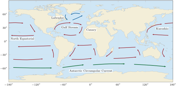
Two features of this pattern need explaining. The first is the sense of rotation: the trade winds blow towards the west on the equatorward side of a subtropical gyre, yet the currents of the gyre do not simply follow the winds, and the surface water drifts at an angle to them. The second is the asymmetry: the return flow of a gyre is crushed against the western side of its basin. Both come from the rotation of the Earth.

29.2 Ekman transport

History — Nansen and Ekman, 1898–1905

During his expedition in the Arctic, Fridtjof Nansen noticed that the wind drove the sea ice not along the wind but at an angle of $20{}^{\circ}$ to $40{}^{\circ}$ to its right, looking downwind. He reasoned that three forces had to balance on the moving ice: the push of the wind, the friction of the water, and the Coriolis force. He asked the meteorologist Vilhelm Bjerknes to let one of his students study the influence of the Earth’s rotation on wind-driven currents. The student, Walfrid Ekman, worked out the theory for his doctoral thesis at Uppsala, and extended it in 1905. His solution is still the starting point of the theory of the wind-driven ocean.

Definition 29.3 (Ekman layer, Ekman transport, Ekman spiral)

The Ekman layer is the thin surface layer of the ocean, at most a few hundred metres thick, in which the stress of the wind is carried down by turbulent friction and balanced by the Coriolis force. The Ekman transport is the mass of water that the layer carries per second across a vertical strip $1\,\mathrm{m}$ wide, from the surface down to below the layer:

$$\vec M = \int_{-d}^{0} \rho\,\vec v\,\mathrm dz \quad (\mathrm{kg}\,\mathrm{m}^{-1}\,\mathrm{s}^{-1});$$

divided by the density, it is a volume transport per metre, in $\mathrm{m}^{2}\,\mathrm{s}^{-1}$. The Ekman spiral is the turning and weakening of the current with depth in the layer. Ocean transports are counted in sverdrups: $1\,\mathrm{Sv}$ $= 10^{6}\,\mathrm{m}^{3}\,\mathrm{s}^{-1}$.

Theorem 29.4 (Ekman transport)

In a steady state, far from coasts, over water much deeper than the Ekman layer, the Ekman transport depends only on the wind stress $\vec T$ and on the Coriolis parameter $f$:

$$\vec M = \frac{1}{f}\,\vec T\times\vec k, \qquad |\vec M| = \frac{|\vec T|}{|f|}.$$

It is at right angles to the wind stress, to its right in the Northern Hemisphere and to its left in the Southern.

The result does not depend on how the friction works inside the layer, which is poorly known: only the stress at the top and its vanishing at the bottom enter. This makes the transport far more robust than the velocities themselves. The water of the whole layer, taken together, moves at right angles to the wind, a result that seems strange until one remembers that over a day or more the Coriolis force has time to turn every current.

Example 29.5 (The transport under a fresh breeze)

A wind of $10\,\mathrm{m}/\mathrm{s}$ blowing towards the north at $35{}^{\circ}$ N exerts $T = 0.170\,\mathrm{Pa}$. With $f = 2\Omega\sin35{}^{\circ} = 8.365 \times 10^{-5}\,\mathrm{s}^{-1}$, the Ekman transport is $0.170/(8.365 \times 10^{-5}) = 2036\,\mathrm{kg}\,\mathrm{m}^{-1}\,\mathrm{s}^{-1}$, towards the east. With $\rho = 1027\,\mathrm{kg}\,\mathrm{m}^{-3}$, this is $1.98\,\mathrm{m}^{3}\,\mathrm{s}^{-1}$ for each metre measured across the transport: across a line $1000\,\mathrm{km}$ long, about $2\,\mathrm{Sv}$.

The theorem has been tested at sea. Across $11{}^{\circ}$ N in the Atlantic, where the trade winds blow towards the west, the Ekman transport is northward; measured directly with a current profiler, it came to $(12.0 \pm 5.5)\,\mathrm{Sv}$, against $(8.8 \pm 1.9)\,\mathrm{Sv}$ computed from the winds measured during the survey and $(13.5 \pm 0.3)\,\mathrm{Sv}$ from winds averaged over many years.

How the current is distributed with depth inside the layer depends on the friction. Ekman took the simplest model, a turbulent friction proportional to the vertical shear of the current, $\vec\tau = \rho A_z\,\partial\vec v/\partial z$, with a constant eddy viscosity $A_z$.

Proposition 29.6 (The Ekman spiral)

For a steady wind stress $T$ towards the north over a deep, homogeneous ocean in the Northern Hemisphere, with a constant eddy viscosity $A_z$, the current at height $z \leq 0$ is

$$u = V_0\,e^{az}\cos\Bigl(\frac\pi4 + az\Bigr),\qquad v = V_0\,e^{az}\sin\Bigl(\frac\pi4 + az\Bigr),\qquad a = \sqrt{\frac{f}{2A_z}},\quad V_0 = \frac{T}{\rho\sqrt{fA_z}},$$

with $u$ eastward and $v$ northward. At the surface the current flows at $45{}^{\circ}$ to the right of the wind; with depth it weakens as $e^{az}$ and turns further to the right. At the depth $D_E = \pi/a$, the Ekman depth, it flows against the surface current with $e^{-\pi} = 0.043$ of its speed.

The derivation solves the two equations $f v + A_z u'' = 0$ and $-f u + A_z v'' = 0$ of the balance in the proof above; it is done in the Year 3 volume, and Exercise 29.10 checks that the formulas satisfy the equations and that the spiral carries exactly the transport of the theorem. To use the spiral, one needs $A_z$, which is not measured directly. Ekman gathered the observed speeds of surface currents and found, for $|\varphi| \geq 10{}^{\circ}$,

in SI units, with his drag coefficient $C_D = 2.6 \times 10^{-3}$ and $\rho_a = 1.25\,\mathrm{kg}\,\mathrm{m}^{-3}$. At $35{}^{\circ}$ N under a wind of $10\,\mathrm{m}/\mathrm{s}$, $D_E = 100\,\mathrm{m}$ and $V_0 = 0.17\,\mathrm{m}/\mathrm{s}$; the Ekman layer ranges from about $45\,\mathrm{m}$ under light winds at mid-latitudes to $300\,\mathrm{m}$ under a gale in the tropics, and the surface current is $1\text{ to }2.5\,\%$ of the wind.

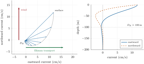
The spiral is an idealisation. Measurements from current meters on moorings and from 1503 drifters followed in the Pacific between 1987 and 1994 show that, averaged over many days, the flow agrees remarkably well with Ekman’s theory: the depth of the layer is almost his, $7.12\,U_{10}/\sqrt{\sin|\varphi|}$; the surface current is about half his value; the angle between the wind and the surface flow is near $45{}^{\circ}$ at mid-latitudes; and the transport is at $90{}^{\circ}$ to the right of the wind. Over a few hours, the picture is blurred by inertial oscillations, and the balance needs the wind to blow steadily for a day or two to establish itself.

29.3 Upwelling and Ekman pumping

Where the Ekman transport is not the same everywhere, water piles up in some places and is drawn away from others; the difference is made up by vertical motion.

Definition 29.7 (Upwelling, downwelling, coastal upwelling)

Upwelling is the rise of water from below into the surface layer of the ocean, to replace surface water carried away; downwelling is the sinking of surface water where it accumulates. Coastal upwelling occurs where a wind blowing along a coast drives an Ekman transport away from the shore: in the Northern Hemisphere, a wind with the coast on its left.

Proposition 29.8 (Coastal upwelling)

Along a straight coast of length $L$, a wind stress of component $T_\parallel$ along the coast, directed so that the Ekman transport points offshore, draws up from below the Ekman layer the volume

$$Q = \frac{T_\parallel\,L}{\rho\,|f|}$$

per second.

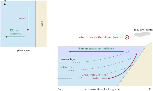
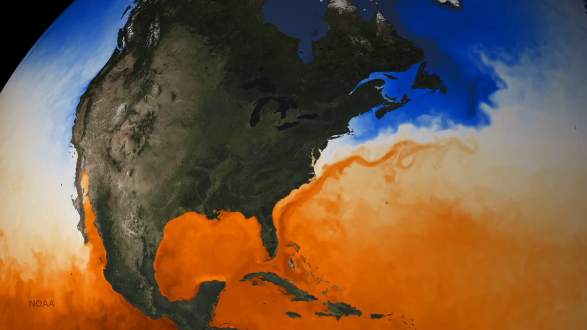
Off California, where the summer winds blow towards the south along the coast, the situation is exactly that of the figure. The upwelled water comes from below the mixed layer: it is colder than the surface water, and richer in nutrients. The nutrients feed the phytoplankton, which feed the zooplankton and the fish: the upwelling regions off Peru, California, Somalia, Morocco and Namibia support some of the world’s main fisheries. The cold water also changes the weather on the coast: the air that crosses it is cooled from below and becomes stably stratified, and such coasts tend to have fog, low stratus clouds, little convection and little rain. The photograph that opens the chapter shows the contrast: the cold water off the Pacific coast of North America, the warm water off the Atlantic coast at the same latitudes.

Upwelling does not need a coast. Along the equator, the trade winds blow towards the west on both sides; just north of the equator their Ekman transport is to the right, northward, and just south of it to the left, southward. The surface water diverges from the equator, and cold water rises along it. In the open ocean, wherever the transport varies from place to place, the same mass balance applies.

Proposition 29.9 (Ekman pumping)

Where the Ekman transport $\vec M$ changes from place to place, water crosses the base of the Ekman layer with the upward velocity

$$w_E = \frac{1}{\rho}\Bigl(\frac{\partial M_x}{\partial x} + \frac{\partial M_y}{\partial y}\Bigr):$$

the water rises where the transports diverge and sinks where they converge.

In a subtropical gyre the trade winds on the equatorward side drive an Ekman transport towards the pole, and the westerlies on the poleward side a transport towards the equator: the two converge, and the surface water is pumped down. Take, for illustration, a stress of $0.08\,\mathrm{Pa}$ towards the west at $15{}^{\circ}$ N and $0.10\,\mathrm{Pa}$ towards the east at $45{}^{\circ}$ N. The transports are $0.08/f(15{}^{\circ}) = 2119\,\mathrm{kg}\,\mathrm{m}^{-1}\,\mathrm{s}^{-1}$ northward and $0.10/f(45{}^{\circ}) = 970\,\mathrm{kg}\,\mathrm{m}^{-1}\,\mathrm{s}^{-1}$ southward. Their convergence over the $3340\,\mathrm{km}$ between the two latitudes gives an average downward velocity of $(2119 + 970)/(1027 \times 3.34 \times 10^{6}) = 9.0 \times 10^{-7}\,\mathrm{m}/\mathrm{s}$, about $28\,\mathrm{m}$ a year. This slow downwelling piles warm surface water into the gyre and deepens its thermocline; the subpolar gyres, under diverging transports, are pumped upwards. How the interior of the ocean responds to this pumping, the Sverdrup balance, is a subject of the Year 3 volume. Around Antarctica, the Ekman transports diverge south of the maximum of the westerlies, near $50{}^{\circ}$ S, and bring Circumpolar Deep Water up to the surface; they converge north of it and push Antarctic Intermediate Water down.

29.4 Western boundary currents

Definition 29.10 (Western boundary current)

A western boundary current is the fast, narrow, poleward current that runs along the western side of an ocean basin and closes its subtropical gyre. The current that closes the gyre on the eastern side, an eastern boundary current, is weak, broad and flows towards the equator.

The Gulf Stream is the western boundary current of the North Atlantic. It comes out of the Gulf of Mexico, leaves through the Strait of Florida, and follows the coast of the United States before turning across the ocean towards Europe. Its average speed is about $6.4\,\mathrm{km}/\mathrm{h}$, $1.8\,\mathrm{m}/\mathrm{s}$, reaching $9\,\mathrm{km}/\mathrm{h}$ near the surface. Through the Strait of Florida it carries $(31.7 \pm 2.2)\,\mathrm{Sv}$ (mean and standard deviation of the monthly values, 2004–2024, measured mainly with an electromagnetic submarine cable), and its transport grows downstream, to about $150\,\mathrm{Sv}$ near $40{}^{\circ}$ N, as it gathers the water of a recirculation south of it. Its path meanders, and the meanders pinch off rings about a degree across; the kinetic energy of these eddies is 8 to 37 times that of the mean flow. In the North Pacific, the Kuroshio plays the same part: it starts east of Luzon, in the Philippines, where the North Equatorial Current divides, flows along the east coast of Taiwan and south of Japan, and also grows as it goes north, from about $16\,\mathrm{Sv}$ at $18.75{}^{\circ}$ N.

History — Stommel 1948

In 1948 Henry Stommel took the simplest ocean he could imagine: a rectangular basin of uniform depth, filled with water of uniform density, driven by a wind blowing towards the west in its southern half and towards the east in its northern half, and slowed by a friction at the bottom proportional to the velocity. Without rotation, or with a uniform rotation, the gyre came out symmetric, with no western boundary current. Only when he let the Coriolis parameter increase towards the north did the streamlines crowd against the western boundary. He suggested that this was the main reason for the Gulf Stream and the other intense currents of the oceans; the explanation, in terms of the spin given to the water by the wind and removed at the western boundary, is part of the Year 3 volume.

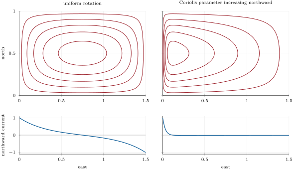
In the computed gyre of the figure above, the fastest northward current at the western boundary is 37 times the southward drift of the interior. In a real ocean the interior drift is too slow to be measured directly against the eddies; Exercise 29.11 estimates both speeds. In the North Atlantic, the theory of the interior predicts a western boundary current of about $30\,\mathrm{Sv}$, largest near $28{}^{\circ}$ N, close to the transport measured in the Strait of Florida; the much larger flow off Cape Hatteras and near $40{}^{\circ}$ N is fed by a recirculation of the Gulf Stream’s own water, south of it.

29.5 The meridional overturning circulation

The wind moves the upper few hundred metres of the ocean. Below, the water of the abyss is renewed by a slow circulation that starts in a few places of the polar oceans, where surface water becomes dense enough to sink to the bottom.

Definition 29.11 (Meridional overturning circulation; thermohaline circulation; deep-water formation)

The meridional overturning circulation (MOC) of an ocean basin is its circulation in the latitude–depth plane, obtained by adding up the northward flow across the whole width of the basin. At a given latitude its strength is the maximum of the overturning streamfunction, the northward transport integrated from the surface down to a given depth, in sverdrups; in the Atlantic it is the AMOC. The older name thermohaline circulation describes the same deep circulation as one driven by differences of temperature and salinity. Deep-water formation is the sinking of surface water, made dense by cooling and by the salt left behind when sea ice forms, to intermediate or abyssal depths.

The name “thermohaline” has almost disappeared from the research literature, for the deep circulation is not driven by density differences alone: the winds that bring deep water up in the Southern Ocean, and the mixing that lifts it elsewhere, are needed to close the loop. The overturning streamfunction is the oceanic counterpart of the streamfunction of Definition 28.11, written in volume rather than mass.

Deep water forms where the surface water is both cold and salty. In winter, the surface water of the far North Atlantic gives its heat to the atmosphere and becomes cold, salty and dense enough to sink in the Greenland and Norwegian Seas, and, as Chapter 26 noted, in the Labrador Sea: this is the source of the North Atlantic Deep Water, which moves south at depths near $2000\,\mathrm{m}$. Around Antarctica, in the shallow Weddell and Ross Seas, the winter freezing of the sea leaves its salt in the water below the ice and produces the coldest and saltiest water of the ocean; it drains off the continental shelves, mixes with the deep water it meets, and spreads along the sea floor as Antarctic Bottom Water, $8\text{ to }10\,\mathrm{Sv}$ of it. Between them, Antarctic Intermediate Water sinks near the Polar Front of the Southern Ocean and spreads north near $1000\,\mathrm{m}$, and the warm, salty water that leaves the Mediterranean spreads through the North Atlantic at intermediate depths. All of these waters can be followed by their temperature and salinity, as Method 26.17 showed.

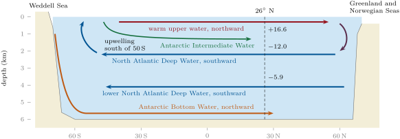
The strength of the Atlantic overturning has been measured continuously since 2004 along $26.5{}^{\circ}$ N, between Florida and Africa. Three pieces are added: the Gulf Stream through the Strait of Florida, $31.7\,\mathrm{Sv}$ northward; the Ekman transport computed from the wind stress, $3.5\,\mathrm{Sv}$ northward; and the flow of the upper water across the open ocean, measured by moorings that record temperature, salinity and pressure from the surface to the sea floor near both boundaries and on either side of the Mid-Atlantic Ridge, $17.9\,\mathrm{Sv}$ southward. Their sum, the northward flow of the upper water across the whole ocean, is the overturning: its mean over April 2004 to November 2024 is $(17.1 \pm 3.2)\,\mathrm{Sv}$, the maximum of the streamfunction lying usually near $1100\,\mathrm{m}$. Below, the Upper North Atlantic Deep Water carries $12.0\,\mathrm{Sv}$ south between 1100 and $3000\,\mathrm{m}$, and the Lower, $5.9\,\mathrm{Sv}$ between 3000 and $5000\,\mathrm{m}$. The array showed that the overturning varies from day to day and from year to year far more than expected, mostly under the influence of the wind; after a major dip in 2010–2011 it has stayed lower, and for short periods it can even reverse.

In the lab — Measuring the deep ocean

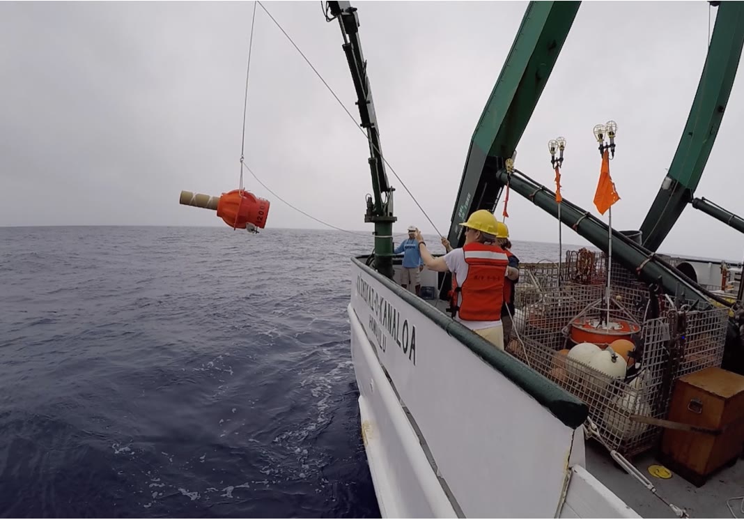
The deep ocean is measured from moorings and floats rather than ships alone. A mooring is an anchored line, reaching from the sea floor towards the surface, carrying instruments that record temperature, salinity, pressure or current until a ship recovers them; a line of such moorings across an ocean, together with an electromagnetic cable across the Strait of Florida and the winds seen from satellites, gives the overturning at $26.5{}^{\circ}$ N. The Argo array keeps nearly $4000$ profiling floats in the ocean: each drifts at depth, then rises to the surface measuring temperature, salinity and pressure on the way, and transmits its profile by satellite about every ten days. The core floats profile down to $2000\,\mathrm{m}$; the floats of Deep Argo, like the one in the photograph below, go down to $6000\,\mathrm{m}$. In 25 years the fleet has collected some three million profiles.

The overturning carries heat. Water that goes north warm and comes back cold has given up heat to the atmosphere of the north.

Proposition 29.12 (Heat carried by an overturning)

If a volume transport $Q$ crosses a latitude northward at the potential temperature $\theta_1$ and returns southward at $\theta_2$, with no net transport of mass, the overturning carries northward the heat flux

$$H = \rho c_p\,Q\,(\theta_1 - \theta_2),$$

where $c_p$ is the specific heat of seawater.

A rough budget of the North Atlantic, by W. Schmitz, has the Gulf Stream carrying $40\,\mathrm{Sv}$ of water at $18\,{}^{\circ}\mathrm{C}$ north, of which $14\,\mathrm{Sv}$ return south as deep water at $2\,{}^{\circ}\mathrm{C}$. With $c_p = 3992\,\mathrm{J}\,\mathrm{kg}^{-1}\,\mathrm{K}^{-1}$ and $\rho = 1027\,\mathrm{kg}\,\mathrm{m}^{-3}$, this overturning carries $1027 \times 3992 \times 14 \times 10^{6} \times 16 = 0.92 \times 10^{15}\,\mathrm{W}$, about $0.9\,\mathrm{PW}$, north of $24{}^{\circ}$ N; careful estimates give $1.2\,\mathrm{PW}$, a quarter of the poleward transport of heat by the atmosphere and the ocean combined. Most of this heat is given to the air over the northern North Atlantic, which is one reason why Norway, at $60{}^{\circ}$ N, is far warmer than southern Greenland at the same latitude.

The deep circulation is slow. If it takes about a thousand years for water sinking in the North Atlantic to reach the North Pacific by way of the Antarctic Circumpolar Current, its mean speed is about $1\,\mathrm{mm}/\mathrm{s}$, a hundred times less than the variable deep currents that a current meter records. Its speed is therefore inferred from tracers rather than measured: tritium, released into the atmosphere by the nuclear tests of the 1950s and decaying with a half-life of 12.3 years, entered the deep North Atlantic where deep water forms, and after 25 years had spread little south of $30{}^{\circ}$ N, a mean speed of less than $1\,\mathrm{mm}/\mathrm{s}$. The volume of the ocean divided by the rate at which deep water forms gives the same order of time (Exercise 29.12).

The Antarctic Circumpolar Current joins the basins. Its currents reach the sea floor and are slow, about $10\,\mathrm{cm}/\mathrm{s}$, up to $50\,\mathrm{cm}/\mathrm{s}$ at its fronts, but it is deep and wide: an array of moored current meters across Drake Passage, between South America and Antarctica, gave $(125 \pm 11)\,\mathrm{Sv}$ (published in 1985), and a denser array in 2007–2011, which measured the currents near the bottom as well, gave $173.3\,\mathrm{Sv}$, $39\,\%$ more than that long-used value. It carries deep water from each ocean to the others and mixes it on the way.

Figures as of 2021

The 2021 assessment of the Intergovernmental Panel on Climate Change finds, from reconstructions, that the Atlantic overturning was relatively stable over the past $8000$ years (medium confidence), with a weakening beginning in the late 19th century (medium confidence), but has only low confidence in an overall decline during the 20th century. The weakening observed directly from the mid-2000s to the mid-2010s (high confidence) cannot be told apart from decade-scale variability (high confidence). The overturning is very likely to weaken over the 21st century for all emissions scenarios, with only low confidence in the size of the decline; there is medium confidence that it will not collapse abruptly before 2100.

29.6 Exercises

Exercise 29.1 ★

Use the bulk formula with $\rho_a = 1.3\,\mathrm{kg}\,\mathrm{m}^{-3}$ and the drag coefficient of Yelland and Taylor. (a) Compute $C_D$ and the wind stress for winds of 4, 7 and $15\,\mathrm{m}/\mathrm{s}$. (b) By what factor does the stress grow from 7 to $15\,\mathrm{m}/\mathrm{s}$? Compare with the ratio of the squares of the speeds and explain the difference.

Solution

Solution of Exercise 29.1.

(a) At $4\,\mathrm{m}/\mathrm{s}$ (first formula): $1000\,C_D = 0.29 + 0.775 + 0.481 = 1.546$, $T = 1.3 \times 1.546 \times 10^{-3} \times 16 = 0.0322\,\mathrm{Pa}$. At $7\,\mathrm{m}/\mathrm{s}$ (second formula): $1000\,C_D = 0.60 + 0.497 = 1.097$, $T = 0.0699\,\mathrm{Pa}$. At $15\,\mathrm{m}/\mathrm{s}$: $1000\,C_D = 1.665$, $T = 0.487\,\mathrm{Pa}$. (b) $0.487/0.0699 = 6.97$, against $(15/7)^2 = 4.59$: the drag coefficient itself grows with the wind, because a stronger wind raises rougher waves that grip the air better.

Exercise 29.2 ★

Give the direction of the Ekman transport in each case. (a) A wind blowing towards the east at $45{}^{\circ}$ N. (b) A trade wind from the north-east at $15{}^{\circ}$ N. (c) A wind blowing towards the east at $50{}^{\circ}$ S. (d) A wind from the south along the west coast of southern Africa, near $23{}^{\circ}$ S. In which of the four cases does the transport point offshore, and what follows?

Solution

Solution of Exercise 29.2.

(a) Northern Hemisphere, $90{}^{\circ}$ to the right of a wind blowing east: towards the south. (b) The wind blows towards the south-west; to its right is the north-west. (c) Southern Hemisphere, $90{}^{\circ}$ to the left of a wind blowing east: towards the north. (d) The wind blows towards the north; to its left is the west, which is offshore on a west coast. In case (d) the transport points offshore: the surface water is replaced from below, and cold water upwells along the coast.

Exercise 29.3 ★

At $26.5{}^{\circ}$ N in the Atlantic, the mean transports of 2004–2024 are: Strait of Florida $31.7\,\mathrm{Sv}$, Ekman $3.5\,\mathrm{Sv}$, upper mid-ocean $-17.9\,\mathrm{Sv}$; by layers, 0–$800\,\mathrm{m}$ $16.6\,\mathrm{Sv}$, 800–$1100\,\mathrm{m}$ $0.4\,\mathrm{Sv}$, 1100–$3000\,\mathrm{m}$ $-12.0\,\mathrm{Sv}$, 3000–$5000\,\mathrm{m}$ $-5.9\,\mathrm{Sv}$ (northward positive). (a) Add the first three and compare with the published overturning, $17.1\,\mathrm{Sv}$. (b) Compare the northward flow above $1100\,\mathrm{m}$ with the southward flow below. (c) Convert $17.1\,\mathrm{Sv}$ into cubic kilometres per year, and compute the time this flow would take to fill the volume of the whole ocean, $1.3324 \times 10^{9}\,\mathrm{km}^{3}$.

Solution

Solution of Exercise 29.3.

(a) $31.7 + 3.5 - 17.9 = 17.3\,\mathrm{Sv}$, against the published $17.1\,\mathrm{Sv}$: the means of the three pieces add up to the mean overturning within the rounding and the uncertainties ($\pm3.2\,\mathrm{Sv}$). (b) Above $1100\,\mathrm{m}$: $16.6 + 0.4 = 17.0\,\mathrm{Sv}$ northward; below: $12.0 + 5.9 = 17.9\,\mathrm{Sv}$ southward. The two nearly balance, as they must when no water accumulates north of the section; the small difference is within the uncertainties. (c) $17.1 \times 10^{6} \times 3.156 \times 10^{7} = 5.40 \times 10^{14}\,\mathrm{m}^{3}$, that is $5.40 \times 10^{5}\,\mathrm{km}^{3}$ a year; $1.3324 \times 10^{9}/(5.40 \times 10^{5}) \approx 2470$ years.

Exercise 29.4 ★

With Ekman’s formulas, compute the Ekman depth and the surface current under a wind of $10\,\mathrm{m}/\mathrm{s}$ at $15{}^{\circ}$, $45{}^{\circ}$ and $60{}^{\circ}$ of latitude, and the surface current as a percentage of the wind. Why do the formulas fail near the equator?

Solution

Solution of Exercise 29.4.

$D_E = 7.6 \times 10/\sqrt{\sin\varphi}$ and $V_0 = 0.0127 \times 10/\sqrt{\sin\varphi}$. At $15{}^{\circ}$: $149\,\mathrm{m}$ and $0.250\,\mathrm{m}/\mathrm{s}$ ($2.5\,\%$ of the wind); at $45{}^{\circ}$: $90\,\mathrm{m}$ and $0.151\,\mathrm{m}/\mathrm{s}$ ($1.5\,\%$); at $60{}^{\circ}$: $82\,\mathrm{m}$ and $0.136\,\mathrm{m}/\mathrm{s}$ ($1.4\,\%$). Near the equator $\sin\varphi \to 0$ and both formulas diverge; more fundamentally $f \to 0$, so that the Coriolis force needed to balance the friction vanishes, and the time $1/f$ the balance needs to set in becomes longer than the winds stay steady. Ekman restricted his formula to $|\varphi| \geq 10{}^{\circ}$.

Exercise 29.5 ★★

Across $11{}^{\circ}$ N in the Atlantic, take a mean wind stress of $0.07\,\mathrm{Pa}$ towards the west over a width of $5000\,\mathrm{km}$, and $\rho = 1027\,\mathrm{kg}\,\mathrm{m}^{-3}$. (a) Compute the Ekman transport per metre and its direction. (b) Compute the total volume transport across the section in sverdrups. (c) Compare with the transports measured directly ($12.0 \pm 5.5\,\mathrm{Sv}$) and computed from long-term winds ($13.5 \pm 0.3\,\mathrm{Sv}$).

Solution

Solution of Exercise 29.5.

(a) $f = 2\Omega\sin11{}^{\circ} = 2.783 \times 10^{-5}\,\mathrm{s}^{-1}$; $M = 0.07/(2.783 \times 10^{-5}) = 2515\,\mathrm{kg}\,\mathrm{m}^{-1}\,\mathrm{s}^{-1}$, $90{}^{\circ}$ to the right of a wind blowing west: northward. (b) $Q = (2515/1027) \times 5 \times 10^{6} = 1.22 \times 10^{7}\,\mathrm{m}^{3}/\mathrm{s}$, $12.2\,\mathrm{Sv}$. (c) The estimate lies within the uncertainty of the direct measurement ($12.0 \pm 5.5$) and close to the value from long-term winds ($13.5 \pm 0.3$): the theorem accounts for the observed transport.

Exercise 29.6 ★★

Along the equatorial Pacific, the trade winds exert a stress of $0.05\,\mathrm{Pa}$ towards the west. (a) Compute the Ekman transport per metre, and its direction, at $2{}^{\circ}$ N and at $2{}^{\circ}$ S. (b) Assuming that the water carried away across these two latitudes is replaced from below between them, compute the mean upwelling velocity in metres per day. (c) What happens to the formula of the theorem at the equator itself? Which conclusion survives?

Solution

Solution of Exercise 29.6.

(a) $f(2{}^{\circ}) = 5.09 \times 10^{-6}\,\mathrm{s}^{-1}$; $M = 0.05/(5.09 \times 10^{-6}) = 9824\,\mathrm{kg}\,\mathrm{m}^{-1}\,\mathrm{s}^{-1}$, $9.57\,\mathrm{m}^{2}/\mathrm{s}$: at $2{}^{\circ}$ N towards the north (right of a westward wind), at $2{}^{\circ}$ S towards the south (left). (b) Over a strip $1\,\mathrm{m}$ long in longitude, $2 \times 9.57 = 19.1\,\mathrm{m}^{3}/\mathrm{s}$ leave across the two latitudes, $444.8\,\mathrm{km}$ apart: $w = 19.1/(4.448 \times 10^{5}) = 4.30 \times 10^{-5}\,\mathrm{m}/\mathrm{s}$, about $3.7\,\mathrm{m}$ a day. (c) At the equator $f = 0$ and $|\vec M| = T/|f|$ is infinite: the steady Ekman balance does not exist there, and the numbers above, very sensitive to the latitude chosen, are only an order of magnitude. What survives is the sign: on either side the transport points away from the equator, so the surface water diverges and cold water rises along it.

Exercise 29.7 ★★

Over a subtropical gyre, take a wind stress of $0.06\,\mathrm{Pa}$ towards the west at $15{}^{\circ}$ N and $0.12\,\mathrm{Pa}$ towards the east at $40{}^{\circ}$ N. (a) Compute both Ekman transports and their directions. (b) Assuming the transport changes uniformly between the two latitudes, compute the vertical velocity at the base of the Ekman layer, in metres per year, and say whether it is upward or downward. (c) Over a basin $5000\,\mathrm{km}$ wide, how many sverdrups are pumped through the base of the layer?

Solution

Solution of Exercise 29.7.

(a) $f(15{}^{\circ}) = 3.775 \times 10^{-5}\,\mathrm{s}^{-1}$: $M = 0.06/(3.775 \times 10^{-5}) = 1590\,\mathrm{kg}\,\mathrm{m}^{-1}\,\mathrm{s}^{-1}$ towards the north; $f(40{}^{\circ}) = 9.375 \times 10^{-5}\,\mathrm{s}^{-1}$: $M = 1280\,\mathrm{kg}\,\mathrm{m}^{-1}\,\mathrm{s}^{-1}$ towards the south. (b) Between the two latitudes, $2780\,\mathrm{km}$ apart, $\partial M_y/\partial y = -(1590 + 1280)/(2.78 \times 10^{6}) = -1.03 \times 10^{-3}\,\mathrm{kg}\,\mathrm{m}^{-2}\,\mathrm{s}^{-1}$: by Proposition 29.9, $w_E = -1.005 \times 10^{-6}\,\mathrm{m}/\mathrm{s}$, a downward velocity of $31.7\,\mathrm{m}$ a year. (c) $1.005 \times 10^{-6} \times 2.78 \times 10^{6} \times 5 \times 10^{6} = 1.40 \times 10^{7}\,\mathrm{m}^{3}/\mathrm{s}$, $14.0\,\mathrm{Sv}$ pumped down.

Exercise 29.8 ★★

Take $\rho = 1027\,\mathrm{kg}\,\mathrm{m}^{-3}$ and $c_p = 3992\,\mathrm{J}\,\mathrm{kg}^{-1}\,\mathrm{K}^{-1}$. (a) Compute the heat carried north by $17\,\mathrm{Sv}$ flowing north at $15\,{}^{\circ}\mathrm{C}$ and returning at $3\,{}^{\circ}\mathrm{C}$. (b) Compare with the $1.2\,\mathrm{PW}$ carried by the Atlantic overturning. (c) If the same water returned south at the surface, along the eastern side of the basin, at $12\,{}^{\circ}\mathrm{C}$, what heat would it carry? What does this say about the importance of deep-water formation?

Solution

Solution of Exercise 29.8.

(a) $H = 1027 \times 3992 \times 17 \times 10^{6} \times 12 = 8.36 \times 10^{14}\,\mathrm{W}$, $0.84\,\mathrm{PW}$. (b) It is $70\,\%$ of the measured $1.2\,\mathrm{PW}$: the real upper limb is warmer near the surface than the mean of $15\,{}^{\circ}\mathrm{C}$, and the gyre also carries heat. (c) $1027 \times 3992 \times 17 \times 10^{6} \times 3 = 2.1 \times 10^{14}\,\mathrm{W}$, $0.21\,\mathrm{PW}$, a quarter of (a). Only water that becomes cold before it returns carries much heat: the heat transport of the Atlantic depends on the formation of deep water.

Exercise 29.9 ★★

Three water masses of the South Atlantic have the potential temperatures and salinities: Antarctic Intermediate Water $3.3\,{}^{\circ}\mathrm{C}$, 34.15; North Atlantic Deep Water $4.0\,{}^{\circ}\mathrm{C}$, 35.00; Antarctic Bottom Water $0.4\,{}^{\circ}\mathrm{C}$, 34.67. A sample at depth has $\theta = 2.78\,{}^{\circ}\mathrm{C}$ and $S = 34.731$. Using Proposition 26.16, find the fraction of each water mass in the sample.

Solution

Solution of Exercise 29.9.

Let $x$, $y$ and $1 - x - y$ be the fractions of AAIW, NADW and AABW. Salt and heat balances, measured from AABW:

$$-0.52\,x + 0.33\,y = 34.731 - 34.67 = 0.061,\qquad 2.9\,x + 3.6\,y = 2.78 - 0.4 = 2.38 .$$

The determinant is $-0.52 \times 3.6 - 0.33 \times 2.9 = -2.829$, and Cramer’s rule gives $x = (0.061 \times 3.6 - 0.33 \times 2.38)/(-2.829) = 0.20$ and $y = (-0.52 \times 2.38 - 2.9 \times 0.061)/(-2.829) = 0.50$: the sample is $20\,\%$ AAIW, $50\,\%$ NADW and $30\,\%$ AABW, a point inside the triangle of the three waters.

Exercise 29.10 ★★★

Take the spiral of Proposition 29.6. (a) Show that $u$ and $v$ satisfy $f v + A_z u'' = 0$ and $-f u + A_z v'' = 0$. (Hint: write $u + iv = V_0\,e^{i\pi/4}\,e^{(1+i)az}$.) (b) Show that the stress $\rho A_z\,\partial\vec v/\partial z$ at the surface equals the wind stress $(0, T)$. (c) Compute the transports $\int_{-\infty}^0 \rho u\,\mathrm dz$ and $\int_{-\infty}^0 \rho v\,\mathrm dz$, and check that they agree with Theorem 29.4.

Solution

Solution of Exercise 29.10.

(a) With $W = u + iv = V_0e^{i\pi/4}e^{(1+i)az}$, whose real and imaginary parts are the formulas of the proposition, $W'' = (1+i)^2a^2W = 2ia^2W$. The two equations combine into $A_z(u'' + iv'') = -fv + ifu = if(u + iv)$, that is $A_zW'' = ifW$, which holds since $2ia^2A_z = if$ for $a^2 = f/(2A_z)$. (b) $W'(0) = (1+i)aV_0e^{i\pi/4} = \sqrt2\,aV_0\,e^{i\pi/2} = i\sqrt2\,aV_0$: the surface stress $\rho A_zW'(0)$ points north, with the size $\rho A_z\sqrt2\,aV_0 = \rho A_z\sqrt2 \sqrt{f/(2A_z)}\;T/(\rho\sqrt{fA_z}) = T$. (c) $\int_{-\infty}^0 W\,\mathrm dz = V_0e^{i\pi/4}/((1+i)a) = V_0/(\sqrt2\,a)$, a real number: the transport has no northward part, and its eastward part is $\rho V_0/(\sqrt2\,a) = T/\sqrt{fA_z}\cdot\sqrt{A_z/f} = T/f$. This is the theorem: size $T/f$, $90{}^{\circ}$ to the right of a wind blowing north.

Exercise 29.11 ★★★

In Stommel’s model, the western boundary current has a width of about $R/\beta$, where $R$ is the rate of bottom friction and $\beta = \mathrm df/\mathrm dy$ the northward rate of increase of the Coriolis parameter. (a) Show that $\beta = 2\Omega \cos\varphi/a_\oplus$ and compute it at $30{}^{\circ}$ N ($a_\oplus = 6371\,\mathrm{km}$). (b) With $R = 10^{-6}\,\mathrm{s}^{-1}$, compute the width. (c) A transport of $30\,\mathrm{Sv}$ drifts south across the interior of a basin $5000\,\mathrm{km}$ wide in the upper $1000\,\mathrm{m}$, and returns north in the boundary current over the same depth. Compute both mean speeds and compare with the speed of the Gulf Stream, $1.8\,\mathrm{m}/\mathrm{s}$.

Solution

Solution of Exercise 29.11.

(a) A northward step $\mathrm dy = a_\oplus\,\mathrm d\varphi$ changes $f = 2\Omega \sin\varphi$ by $2\Omega\cos\varphi\,\mathrm d\varphi$, so $\beta = 2\Omega \cos\varphi/a_\oplus = 2 \times 7.292 \times 10^{-5} \times \cos30{}^{\circ}/(6.371 \times 10^{6}) = 1.98 \times 10^{-11}\,\mathrm{m}^{-1}\,\mathrm{s}^{-1}$. (b) $R/\beta = 10^{-6}/(1.98 \times 10^{-11}) = 5.04 \times 10^{4}\,\mathrm{m}$, about $50\,\mathrm{km}$. (c) Interior: $30 \times 10^{6}/(5 \times 10^{6} \times 1000) = 6.0 \times 10^{-3}\,\mathrm{m}/\mathrm{s}$, $6\,\mathrm{mm}/\mathrm{s}$; boundary current: $30 \times 10^{6}/(5.04 \times 10^{4} \times 1000) = 0.60\,\mathrm{m}/\mathrm{s}$, a hundred times faster, the ratio of the widths. The Gulf Stream, at $1.8\,\mathrm{m}/\mathrm{s}$, is faster still: the real current is narrower than this estimate, its flow is concentrated near the surface, and its recirculation adds to its transport.

Exercise 29.12 ★★★

The ocean holds $1.3324 \times 10^{9}\,\mathrm{km}^{3}$ over $361.84 \times 10^{6}\,\mathrm{km}^{2}$. (a) Show that the volume below $1000\,\mathrm{m}$ is at least $9.71 \times 10^{8}\,\mathrm{km}^{3}$. (b) North Atlantic Deep Water forms at about $17\,\mathrm{Sv}$ and Antarctic Bottom Water at about $9\,\mathrm{Sv}$. Estimate the time needed to renew the water below $1000\,\mathrm{m}$, and compare with the thousand years of the conveyor. (c) Tritium has a half-life of 12.3 years. What fraction of a tritium input remains after 25 years? How far does water moving at $1\,\mathrm{mm}/\mathrm{s}$ travel in 25 years?

Solution

Solution of Exercise 29.12.

(a) Wherever the sea is deeper than $1000\,\mathrm{m}$, the column above $1000\,\mathrm{m}$ holds at most $1\,\mathrm{km}$ of water, and elsewhere less: the volume above $1000\,\mathrm{m}$ is at most $361.84 \times 10^{6} \times 1 = 3.618 \times 10^{8}\,\mathrm{km}^{3}$, so the volume below is at least $1.3324 \times 10^{9} - 3.618 \times 10^{8} = 9.71 \times 10^{8}\,\mathrm{km}^{3}$. (b) $26 \times 10^{6} \times 3.156 \times 10^{7} = 8.21 \times 10^{14}\,\mathrm{m}^{3}$ a year, $8.21 \times 10^{5}\,\mathrm{km}^{3}$; $9.71 \times 10^{8}/(8.21 \times 10^{5}) \approx 1200$ years, the same order as the thousand years of the conveyor. (c) $(1/2)^{25/12.3} = 0.244$, about a quarter; $10^{-3} \times 25 \times 3.156 \times 10^{7} = 7.9 \times 10^{5}\,\mathrm{m}$, about $790\,\mathrm{km}$. After 25 years the tritium has spread no farther than a slow drift would carry it, while a quarter of it is left to be detected.

29.7 Problem: An upwelling coast

Problem 29.1

Weekend problem — a summer wind along a coast at $38{}^{\circ}$ N

A straight coast runs north–south at $38{}^{\circ}$ N, with the ocean to the west. In summer, a steady wind of $8\,\mathrm{m}/\mathrm{s}$ blows from the north along it for weeks. The coast is invented, but its numbers are typical of the eastern sides of the oceans. Use $\Omega = 2\pi/(23.9345\,\mathrm{h})$, $\rho_a = 1.3\,\mathrm{kg}\,\mathrm{m}^{-3}$, the drag coefficient of Yelland and Taylor, $\rho = 1027\,\mathrm{kg}\,\mathrm{m}^{-3}$ for seawater and $c_p = 3992\,\mathrm{J}\,\mathrm{kg}^{-1}\,\mathrm{K}^{-1}$.

Part I — The wind and its stress.

1. Towards which direction does the wind blow? Is it along the coast or across it?
2. Compute the drag coefficient.
3. Compute the wind stress.
4. Same two questions for a wind of $12\,\mathrm{m}/\mathrm{s}$. By what factor does the stress grow, and why is it more than the ratio of the squares of the speeds?
5. Compute the Coriolis parameter at $38{}^{\circ}$ N.
6. Compute $2\pi/f$ in hours. Why must the wind blow for a day or more before the Ekman balance applies?

Part II — The Ekman layer.

7. In which direction is the Ekman transport? Towards the land or the open sea?
8. Compute the Ekman mass transport per metre of coast.
9. Convert it into a volume transport per metre.
10. Compute the Ekman depth with Ekman’s formula.
11. Compute the mean offshore velocity in the layer, in $\mathrm{cm}/\mathrm{s}$.
12. Compute the surface current with Ekman’s formula, and its direction. What do the drifter measurements suggest instead for its speed?

Part III — Upwelling at the coast.

13. Explain, with a sketch of a vertical section, where the water carried offshore comes from.
14. Compute the volume upwelled per day along each kilometre of coast.
15. Suppose the water rises through a band $20\,\mathrm{km}$ wide along the coast. Compute the mean upward velocity, in $\mathrm{m}/\mathrm{s}$ and in metres per day.
16. How long does water take to rise from the base of the Ekman layer to the surface at this speed?
17. The upwelled water reaches the surface at $12\,{}^{\circ}\mathrm{C}$, while the open sea offshore is at $18\,{}^{\circ}\mathrm{C}$. The sea breeze carries warm, moist air from offshore over this water. What happens to the air near the surface, and what weather follows on the coast?
18. Why are such coasts rich in fish?
19. In autumn the wind turns and blows from the south for a week. What happens to the transport and to the water at the coast?

Part IV — Other coasts and the total transport.

20. With the same stress, compute the Ekman transport per metre at $20{}^{\circ}$ N and compare with $38{}^{\circ}$ N.
21. On the west coast of southern Africa, near $23{}^{\circ}$ S, which wind direction drives upwelling? Compare with the coast of the problem.
22. Under a wind of $5\,\mathrm{m}/\mathrm{s}$ instead of $8\,\mathrm{m}/\mathrm{s}$ at $38{}^{\circ}$ N, compute the stress and the Ekman transport per metre, and their ratio to those of question 8.
23. The upwelled water warms by $6\,{}^{\circ}\mathrm{C}$ as it drifts offshore. Compute the heat it takes up per second per metre of coast, then along $1000\,\mathrm{km}$.
24. What length of such a coast would upwell as much water as the Gulf Stream carries through the Strait of Florida, $31.7\,\mathrm{Sv}$?
25. What volume of water, in sverdrups, is upwelled along $1000\,\mathrm{km}$ of this coast?

Solution

Solution of Problem 29.1.

1. A wind from the north blows towards the south, along the coast.
2. $1000\,C_D = 0.60 + 0.071 \times 8 = 1.168$: $C_D = 1.168 \times 10^{-3}$.
3. $T = 1.3 \times 1.168 \times 10^{-3} \times 64 = 0.0972\,\mathrm{Pa}$.
4. $C_D = 1.452 \times 10^{-3}$ and $T = 0.272\,\mathrm{Pa}$: the stress grows by $2.80$, more than $(12/8)^2 = 2.25$, because $C_D$ itself increases with the wind.
5. $\Omega = 7.292 \times 10^{-5}\,\mathrm{rad}\,\mathrm{s}^{-1}$; $f = 2\Omega\sin38{}^{\circ} = 8.979 \times 10^{-5}\,\mathrm{s}^{-1}$.
6. $2\pi/f = 7.00 \times 10^{4}\,\mathrm{s}$, $19.4\,\mathrm{h}$. The Coriolis force turns a current through a full circle in this time; before the wind has blown for about that long, the water oscillates instead of settling into the steady balance of the theorem.
7. $90{}^{\circ}$ to the right of a wind blowing south: towards the west, the open sea.
8. $M = T/f = 0.0972/(8.979 \times 10^{-5}) = 1082\,\mathrm{kg}\,\mathrm{m}^{-1}\,\mathrm{s}^{-1}$.
9. $1082/1027 = 1.054\,\mathrm{m}^{2}/\mathrm{s}$ for each metre of coast.
10. $D_E = 7.6 \times 8/\sqrt{\sin38{}^{\circ}} = 77.5\,\mathrm{m}$.
11. $1.054/77.5 = 0.0136\,\mathrm{m}/\mathrm{s}$, $1.36\,\mathrm{cm}/\mathrm{s}$.
12. $V_0 = 0.0127 \times 8/\sqrt{\sin38{}^{\circ}} = 0.129\,\mathrm{m}/\mathrm{s}$, $45{}^{\circ}$ to the right of the wind: towards the south-west. The drifters give about half of Ekman’s value, some $0.07\,\mathrm{m}/\mathrm{s}$.
13. The water leaving the coast in the Ekman layer cannot be replaced across the coast, nor from above: it is replaced by water rising from below the layer near the coast, as in the cross-section drawn in Section 29.3; the isotherms bend up towards the shore.
14. $1.054 \times 1000 \times 86400 = 9.11 \times 10^{7}\,\mathrm{m}^{3}$ a day per kilometre of coast.
15. $w = 1.054/(2 \times 10^{4}) = 5.27 \times 10^{-5}\,\mathrm{m}/\mathrm{s}$, $4.55\,\mathrm{m}$ a day.
16. $77.5/4.55 = 17$ days.
17. The air is cooled from below by the cold water: the layer near the surface becomes cold and stable, the moisture may condense into fog and low stratus, and with no convection there is little rain on the coast.
18. The upwelled water is rich in nutrients; they feed the phytoplankton, which feed the zooplankton and the fish.
19. A wind blowing north drives a transport $90{}^{\circ}$ to its right, towards the east: surface water piles up against the coast and sinks (downwelling); the upwelling stops and warmer surface water returns to the coast.
20. $f(20{}^{\circ}) = 4.988 \times 10^{-5}\,\mathrm{s}^{-1}$: $M = 1948\,\mathrm{kg}\,\mathrm{m}^{-1}\,\mathrm{s}^{-1}$, $\sin38{}^{\circ}/\sin20{}^{\circ} = 1.80$ times more.
21. In the Southern Hemisphere the transport is $90{}^{\circ}$ to the left of the wind. To push it west, offshore, the wind must blow towards the north, from the south: in both cases the wind blows along the coast towards the equator.
22. $1000\,C_D = 0.29 + 0.62 + 0.308 = 1.218$; $T = 0.0396\,\mathrm{Pa}$; $M = 441\,\mathrm{kg}\,\mathrm{m}^{-1}\,\mathrm{s}^{-1}$; the ratio is $0.407$ for both.
23. Per metre of coast, $M c_p\,\Delta T = 1082 \times 3992 \times 6 = 2.59 \times 10^{7}\,\mathrm{W}$, $25.9\,\mathrm{MW}$; along $1000\,\mathrm{km}$, $2.59 \times 10^{13}\,\mathrm{W}$, $25.9\,\mathrm{TW}$.
24. $31.7 \times 10^{6}/1.054 = 3.01 \times 10^{7}\,\mathrm{m}$, about $30\,000\,\mathrm{km}$: coastal upwelling moves far less water than a western boundary current.
25. $Q = 1.054 \times 10^{6} = 1.05 \times 10^{6}\,\mathrm{m}^{3}/\mathrm{s}$: the upwelling transport along $1000\,\mathrm{km}$ of coast is $1.05\,\mathrm{Sv}$.