21Clastic Sediments and Their Environments

Pick up a handful of sand on a beach and let it run through your fingers: the grains are all nearly the same size, rounded and clean, and they flow like water. A few hundred kilometres inland, at the foot of a hill left by an old glacier, the ground is a stiff mixture of boulders, pebbles, sand and mud, without order. The two deposits are made of the same kind of debris, broken from the same kinds of rock; what separates them is how the grains travelled and where they came to rest. A wave that runs up and down a beach thousands of times a day sorts the grains by size, carries the fine ones away and rounds the rest; ice carries everything it picks up and drops it all together when it melts. This chapter learns to read such stories from the grains themselves, from the structures they build on the beds of rivers and seas, and from the order in which the deposits are stacked.

You already know

A sediment is loose material laid down by water, wind or ice, and over time sediments pile up in layers that harden into sedimentary rock (Book 1, grades 6 and 7). A river that swings from side to side across its floodplain forms meanders; where it enters the sea or a lake and drops its load, it builds a delta; waves pile sand into beaches and move it along the shore by longshore drift (Book 1, grades 5 and 9). A river carries its load as bed load, suspended load and dissolved load; a grain sinks at its settling velocity; it starts to move when the bed shear stress passes its threshold of motion, and the Hjulström diagram shows the mean velocities of erosion, transport and deposition against the grain size (Chapter 20). The vector mean of a set of directions is the direction of the sum of their unit vectors (Definition 6.4).

21.1 Grain size and sorting

The size of the grains is the first thing a geologist records in a clastic sediment, one made of fragments of older rocks, because it measures the energy of the current that laid them down. Grain sizes in nature span more than seven orders of magnitude, from boulders metres across to clay particles a thousandth of a millimetre wide, and they are measured on a scale of ratios.

Definition 21.1 (Grain-size scale, phi scale)

The grain-size scale of sedimentology divides the diameters of grains into classes whose limits double from one class to the next, starting from $1\,\mathrm{mm}$; each class is named (sand, silt…). The phi scale expresses a diameter $d$ by

$$\varphi = -\log_2 \frac{d}{1\,\mathrm{mm}},$$

so that $d = 2^{-\varphi}$ mm: $1\,\mathrm{mm}$ is $\varphi = 0$, $2\,\mathrm{mm}$ is $\varphi = -1$, $0.25\,\mathrm{mm}$ is $\varphi = 2$, and finer grains have larger values of $\varphi$.

On the phi scale every class of the grain-size scale is one unit wide: a class running from $d$ to $2d$ runs from $\varphi$ to $\varphi - 1$. The main classes, with the names in common use, are listed in Table 21.1.

class	diameter ($\mathrm{mm}$)	$\varphi$
boulder	above 256	below $-8$
cobble	64 to 256	$-6$ to $-8$
pebble	4 to 64	$-2$ to $-6$
granule	2 to 4	$-1$ to $-2$
sand (very coarse, coarse, medium, fine, very fine)	$1/16$ to 2	4 to $-1$
silt (coarse, medium, fine, very fine)	$1/256$ to $1/16$	8 to 4
clay	below $1/256$ ($3.9\,\text{µ}\mathrm{m}$)	above 8

The word clay has two meanings in this book: here it is a size class, in Chapter 19 a family of minerals. Most clay-sized particles are clay minerals and most clay minerals are clay-sized, but the two do not coincide: quartz ground very fine is clay-sized, and a kaolinite book can be the size of silt.

Measuring the sizes. Gravel is measured grain by grain with calipers. Sand is sieved: a stack of sieves with meshes at every whole or half phi unit is shaken, and each sieve’s catch is weighed. Silt and clay, finer than $4\,\varphi$, are measured by settling: the sediment is stirred into water, and since each grain sinks at a speed set by its size (Stokes’ law, Proposition 20.5), the mass still in suspension at a given depth and time tells how much of the sample is finer than a given diameter. Laser instruments that measure the scattering of light by the grains are now common too. The result is a list of the weight per cent in each class.

Definition 21.2 (Mean grain size, sorting)

Let the grain sizes of a sediment, in phi units, have the distribution given by the weight in each class. Its mean grain size is the mean of that distribution, and its sorting is the spread of the distribution, measured by its standard deviation in phi units: a sediment is well sorted when its grains are nearly all of one size, and poorly sorted when they cover many classes. Both are computed either from the percentages in the classes, by the method of moments, or from the cumulative curve, by the graphic measures of Folk:

$$M_z = \frac{\varphi_{16} + \varphi_{50} + \varphi_{84}}{3}, \qquad \sigma_I = \frac{\varphi_{84} - \varphi_{16}}{4} + \frac{\varphi_{95} - \varphi_{5}}{6.6},$$

where $\varphi_p$ is the size in phi units than which $p$ per cent of the sample is coarser.

Method 21.3 (Mean and sorting from a sieve analysis)

1. List the weight per cent $w_i$ in each class, from the coarsest to the finest, and check that the sum is $100\,\%$ (or divide by it).
2. Method of moments. With $x_i$ the mid-point of class $i$ in phi units, compute the mean $m = \sum w_i x_i / 100$ and the standard deviation $s = \sqrt{\sum w_i (x_i - m)^2 / 100}$.
3. Graphic measures. Accumulate the percentages to get the weight per cent coarser than each class limit, and plot it against $\varphi$: this is the cumulative curve.
4. Read on it, by linear interpolation between class limits, the sizes $\varphi_5$, $\varphi_{16}$, $\varphi_{50}$, $\varphi_{84}$ and $\varphi_{95}$.
5. Compute $M_z$ and $\sigma_I$ (Definition 21.2), convert $M_z$ to millimetres by $d = 2^{-M_z}$, and name the sorting from the scale below.

The two methods give nearly the same answers, and the reason is the following property.

Proposition 21.4 (Graphic measures of a normal distribution)

If the sizes of a sediment, in phi units, are distributed normally with mean $\mu$ and standard deviation $\sigma$, then $M_z = \mu$ and $\sigma_I = 0.996\,\sigma$.

The constant 6.6 in Folk’s formula is chosen for this: the interval from the 5th to the 95th percentile spans $3.29$ standard deviations of a normal distribution, and the formula averages the estimates of $\sigma$ from the two intervals, $(\varphi_{84}-\varphi_{16})/2$ and $(\varphi_{95}-\varphi_5)/3.3$. Using the tails as well as the central two-thirds of the curve makes $\sigma_I$ sensitive to the coarse and fine admixtures that tell the most about how a sediment was deposited.

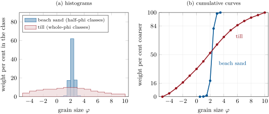
Words for the sorting. From many measured sediments Folk proposed a verbal scale for $\sigma_I$: below $0.35$ very well sorted, $0.35$ to $0.50$ well sorted, $0.50$ to $0.71$ moderately well sorted, $0.71$ to $1.0$ moderately sorted, $1.0$ to $2.0$ poorly sorted, $2.0$ to $4.0$ very poorly sorted, and above $4.0$ extremely poorly sorted. The best sorting attained by natural sediments is about $0.20$ to $0.25$, and the sands of dunes and beaches he measured were between $0.25$ and $0.35$; river sediments ranged from $0.40$ to $2.5$, the silts and clays of floodplains and shelves from about $2.0$ to $3.5$, and the most poorly sorted of all were glacial tills and mudflows. The beach sand of the figure, at $0.36$, is well sorted, on the edge of very well sorted; the till, at $3.84$, very poorly sorted. In the till the method of moments gives a mean of $1.89\,\varphi$ and a standard deviation of $3.64\,\varphi$, close to the graphic values; the differences come from the tails and the asymmetry of the distribution.

The sorting is a record of the transport. A current sorts its load because the grains it can move, and keep in suspension, depend on their size (Section 20.3): waves on a beach and wind over a dune work the same grains again and again, removing the finer ones and leaving behind those too heavy to move, and their deposits are the best sorted of all. Ice, debris flows and the sudden dumping of a flood sort nothing.

Shape and roundness. The roundness of a grain describes the sharpness of its corners, independently of its overall shape: Wadell defined it as the mean radius of curvature of the corners divided by the radius of the largest circle inscribed in the grain’s outline, from 1 for a ball down to near 0 for a splinter. Measuring it is tedious, and grains are compared instead with charts of photographs; on Wadell’s scale most sand grains have roundnesses of $0.3$ to $0.4$, and on the logarithmic scale of Folk, from 0 (very angular) to 6 (very round), about $2.5$, subangular. Rounding is slow for sand: wind-blown quartz rounds much faster than quartz carried by water, which cushions the impacts, and beach sand faster than river sand, while sand grains are hardly rounded in rivers at all. Pebbles round quickly in rivers, the soft ones first: on the Colorado River, limestone pebbles reach their final roundness within a few miles, while quartz pebbles need about 150 miles to catch up.

Definition 21.5 (Textural maturity, compositional maturity)

The textural maturity of a sand or sandstone measures how far the sorting, abrasion and winnowing of the current have worked on it, in four stages: immature, with more than $5\,\%$ of clay matrix; submature, with less clay but poorly sorted grains ($\sigma > 0.5\,\varphi$); mature, with little or no clay and well-sorted ($\sigma < 0.5\,\varphi$) but angular grains; supermature, with no clay and grains both well sorted and well rounded. Its compositional maturity measures how far the unstable minerals and rock fragments have been removed, leaving quartz: it is high in a sandstone of nearly pure quartz and low in one rich in feldspar, mica or fragments of rock.

Textural maturity is read from the deposit as it was laid down: clay minerals that crystallised later in the pores, and the cements that bind the grains (Chapter 23), do not count. It reflects the energy of the place of deposition: immature sediments accumulate on floodplains, alluvial fans and in lagoons, where currents are weak or deposition too fast for the grains to be worked, and supermature ones on beaches and in desert dunes, where energy is spent on the grains without end. Compositional maturity follows from abrasion and from weathering together. Feldspar, softer than quartz and with a good cleavage, is worn down faster; an arkose of angular quartz and feldspar of the same size can, by abrasion alone, end as a supermature sandstone in which the sand is nearly all quartz and the feldspar survives only as silt. Weathering, in the source area and during long storage on the way, does the same by turning feldspars into clay (Section 19.2). Sandstones laid down in times of crustal unrest, quickly eroded from rising mountains, tend to be immature in both senses; those of quiet times, reworked for long, tend to be supermature quartz sandstones; but exceptions are many, and any composition can occur at any stage of textural maturity.

21.2 Bedforms and sedimentary structures

When a current moves sand over a bed, the bed rarely stays flat: it organises itself into waves of sand that travel with the flow. These shapes, and the layering they leave inside the deposit, are the most direct record of the currents of the past.

Definition 21.6 (Bedform, ripple, dune)

A bedform is a regular relief moulded by a current on a bed of loose grains, repeated along the flow. A ripple is a small bedform, a few centimetres high and 10 to $20\,\mathrm{cm}$ from crest to crest, with a gentle upstream (stoss) side and a steep downstream (lee) side; a dune has a similar shape but is at least ten times larger, from decimetres to metres high under water.

The stoss side of a ripple slopes at less than about $10{}^{\circ}$; its lee side, the slip face, stands near the angle of repose of sand in water, about $30{}^{\circ}$. Sand is eroded from the stoss side, carried over the crest, and avalanches down or rains onto the slip face, so the whole ripple moves downstream, far more slowly than the water, by taking grains from its back and adding them to its front. Wind builds ripples and dunes of the same kind on land, the dunes of deserts far larger than those of rivers.

Proposition 21.7 (Bedform migration and bed load)

A train of bedforms of triangular profile, of height $H$, moving downstream at the speed $c$ without changing shape, by erosion of the stoss sides and deposition on the lee sides, carries over the crests the volume of bed load per unit width and time

$$q_b = (1 - p)\,\frac{c\,H}{2},$$

counted as solid grains, where $p$ is the porosity of the sand.

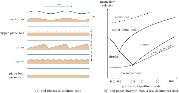
The sequence of bed phases. In a laboratory flume with a bed of medium sand, an increasing flow builds a fixed succession of bed configurations. Below the threshold of motion the bed stays flat. Just above it ripples appear; at a velocity that is a moderate fraction of a metre per second they are replaced, over a few centimetres per second, by dunes. Faster still, the dunes flatten, and the bed becomes a plane again, the upper plane bed, over which sand moves in a dense sheet and in suspension. Finally, when the mean velocity $U$ approaches the speed $\sqrt{gh}$ of surface waves in water of depth $h$, that is when the Froude number $U/\sqrt{gh}$ approaches 1, the water surface and the bed form waves in phase, which grow, steepen, break and form again: antidunes, named by G. K. Gilbert in his flume experiments of 1914, because their crests move upstream. Antidunes need shallow, fast flows and are unimportant in flows deeper than a few metres.

The grain size changes the sequence. Ripples form only in sand finer than about $0.8\,\mathrm{mm}$; in coarse sand and gravel the bed passes from a plane bed without motion to a lower plane bed with moving grains and then directly to dunes. In fine sand, below about $0.2\,\mathrm{mm}$, the dunes never form, and the ripples give way directly to the upper plane bed. The fields of the bed phases are mapped on diagrams of velocity against grain size, drawn for a given depth of flow.

Definition 21.8 (Cross-bedding, palaeocurrent)

Cross-bedding is a layering inclined to the main bedding, made of the successive lee faces (foresets) of migrating ripples or dunes, in units, the sets, bounded by erosion surfaces; cross-bedding made by ripples, in sets a few centimetres thick, is called cross-lamination. A palaeocurrent is the direction of an ancient current, inferred from the structures it left: the foresets dip downstream, so the direction of dip of the cross-beds, once the bedding is restored to the horizontal, is the direction toward which the current flowed.

Proposition 21.9 (Climbing bedforms)

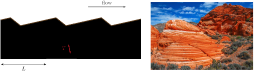
A train of identical bedforms, spaced at $L$ and moving downstream at the speed $c$ while the bed is raised by deposition at the rate $a$, climbs along paths inclined at the angle $\theta$ to the bed, with

$$\tan\theta = \frac{a}{c}.$$

The deposit is then a stack of cross-bedded sets of thickness, measured perpendicular to the set boundaries,

$$T = L\,\sin\theta .$$

When $a = 0$, nothing of the foresets is preserved.

The climbing angle is small for most dunes and ripples, which is why a set preserves only the lower part of the foresets, cut off at the top by the next erosion surface: the truncated tops and the tangential, curving bases of cross-beds tell which way was up, one of the criteria used to tell whether a sequence of beds is the right way up or overturned (Chapter 17). Where sand rains out of suspension fast, as in a waning flood, the angle of climb becomes steep and whole ripple profiles are preserved, stacked as climbing ripples.

Palaeocurrents. The dip directions of cross-beds measured on an outcrop scatter around the mean direction of the current, because the lee faces of dunes and ripples are curved and the currents themselves wander. Their mean is taken as a vector mean, not an arithmetic one, for the reason shown in Proposition 6.5: azimuths are angles on a circle, and 350 and 010 average to 000, not 180.

Proposition 21.10 (Mean of azimuths)

Let $\alpha_1, \ldots, \alpha_N$ be azimuths, measured clockwise from north. Their vector mean $\bar\alpha$ and their mean resultant length $\bar R$ are given by

$$S = \sum_{i=1}^N \sin\alpha_i, \quad C = \sum_{i=1}^N \cos\alpha_i, \quad \bar\alpha = \operatorname{atan2}(S, C), \quad \bar R = \frac{\sqrt{S^2 + C^2}}{N},$$

where $\operatorname{atan2}(S, C)$ is the angle whose sine and cosine are proportional to $S$ and $C$, taken between $0{}^{\circ}$ and $360{}^{\circ}$. $\bar R$ lies between 0 and 1, and is 1 only if all the azimuths are equal.

Method 21.11 (Palaeocurrent from cross-bedding)

1. On each set, measure the dip direction of the foresets, choosing surfaces that show their true dip (or measure strike and dip).
2. Measure the attitude of the main bedding; if it is tilted by more than a few degrees, rotate each foreset back to the horizontal about the strike of the bedding (a rotation done with the stereographic projection of the Year 3 volume).
3. Compute the vector mean $\bar\alpha$ and $\bar R$ of the corrected dip directions (Proposition 21.10).
4. Plot the readings as a rose diagram, a circular histogram of azimuths, to see whether they form one group or two: tidal currents that reverse build sets that dip in opposite directions, in herringbone cross-bedding, and a single mean is then meaningless.

Other structures. Several other structures record the conditions of deposition and the way up of the beds. A graded bed fines upward, from coarse at its base to fine at its top, as grains settle from a waning current, the coarsest first (Definition 21.15). Mud cracks, polygons of shrinkage cracks filled by the next layer, form where mud dries in the air, as on tidal flats and floodplains. Scours cut by the current into the mud below, and filled by the sand above, are preserved as casts on the base of the sandstone bed, and their shapes point the way the current went.

21.3 Facies, rivers and deltas

Grain size, sorting, structures, fossils and composition together make the character of a sedimentary rock, and geologists use one word for that character.

Definition 21.12 (Sedimentary facies, depositional environment)

A sedimentary facies is a body of sedimentary rock distinguished from others by its lithology, grain size, sedimentary structures and fossils, all of which reflect the conditions under which it was formed. The depositional environment is the place, with its physical, chemical and biological conditions, in which a sediment is laid down: a river channel, a floodplain, a beach, the slope of a delta, the deep sea floor.

A facies is a description, an environment an interpretation, and several environments can make the same facies: rippled sand is laid down in rivers, on tidal flats and on the deep sea floor. The interpretation therefore rests on associations of facies and on the order in which they are stacked, which follow the movement of the environments in space: the general laws of that stacking, and the standard models of each environment, are the subject of the Year 3 volume. This chapter describes the main clastic environments and the vertical successions that identify them.

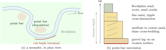
Braided and meandering rivers. Rivers come in two main styles. A braided river flows in many channels that split and rejoin around bars of gravel and sand; braided rivers carry coarse loads near their sources, below mountains or in front of glaciers, and their deposits are sheets of gravel and coarse, cross-bedded sand, with little mud. A meandering river flows in a single sinuous channel. The fastest water runs along the outside of each bend, where it erodes the cut bank; on the inside, where the water is slowest, sand is laid down on the point bar. The meander thus migrates sideways, eroding on one side and building on the other; the floodplain beyond the banks receives only the mud of the floods.

The succession of the point bar follows from the bedforms. At the foot of the bar, in the deepest and fastest water, the current leaves the coarsest grains and builds dunes; up the gently sloping bar the water becomes shallower and slower, the sand finer and the dunes give way to ripples (Section 21.2); at the top, the bar passes into the floodplain. As the bend migrates, each of these zones moves over the one below it, and a borehole through the deposit meets them stacked: a fining-upward succession from an erosion surface to mud, one for each passage of a channel, whose thickness is about the depth of the channel that made it.

Deltas. Where a river enters a standing body of water, its current spreads and slows, and its load is dropped: the coarse load near the mouth, the fine load farther out. A delta grows forward, or progrades, as long as the river supplies more sediment than the waves and tides can carry away. What the waves and the tides do to the supply decides its shape.

Definition 21.13 (River-, wave- and tide-dominated deltas)

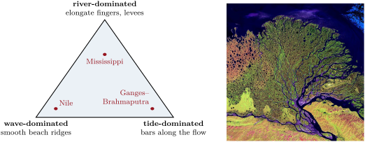
A delta is river-dominated when the river’s supply overwhelms the waves and tides, and its distributary channels, confined by their own levees, build long fingers of sand into the sea; it is wave-dominated when waves rework the sand brought to the mouths into beaches and beach ridges along a smooth, arched coast; it is tide-dominated when tidal currents, flowing in and out of the mouths, shape its sand into bars and ridges parallel to the flow, separated by funnel-shaped channels.

The three end members are the corners of a triangle in which any delta can be placed by the relative strength of the three processes. The bird’s-foot delta of the Mississippi, with its long fingers into the Gulf of Mexico (Chapter 20), is the classic river-dominated delta; the Nile, with its smooth arc of beaches, a wave-dominated one; the delta of the Ganges and Brahmaputra, the largest in the world, a tide-dominated one.

The coarsening-upward succession. In front of the river mouth, the delta has a gently sloping front, the delta front, which passes seaward into the prodelta, where only mud settles from suspension. As the delta progrades, each of these zones advances over the one in front of it: a borehole on the delta plain meets, from bottom to top, the laminated muds of the prodelta, then alternating silt and sand of the lower delta front, then the cross-bedded sand of the mouth bars, cut at the top by the channels of the delta plain. The succession coarsens upward, the reverse of a point bar, and its thickness is about the depth of water into which the delta built. Its rate is linked to the geometry of the delta front.

Proposition 21.14 (Progradation and accumulation)

Let a delta front of constant slope $\alpha$ advance horizontally at the speed $v$ without changing shape, at constant sea level. A fixed point under the front then receives sediment at the vertical rate

$$a = v\,\tan\alpha,$$

and the delta-front succession of thickness $h$ accumulates there in the time $h/(v\tan\alpha)$.

Delta fronts slope gently, so $\tan\alpha$ is small: the front of a delta advances far faster than the sediment piles up at any point under it (Exercise 21.12).

In the lab — Describing a core

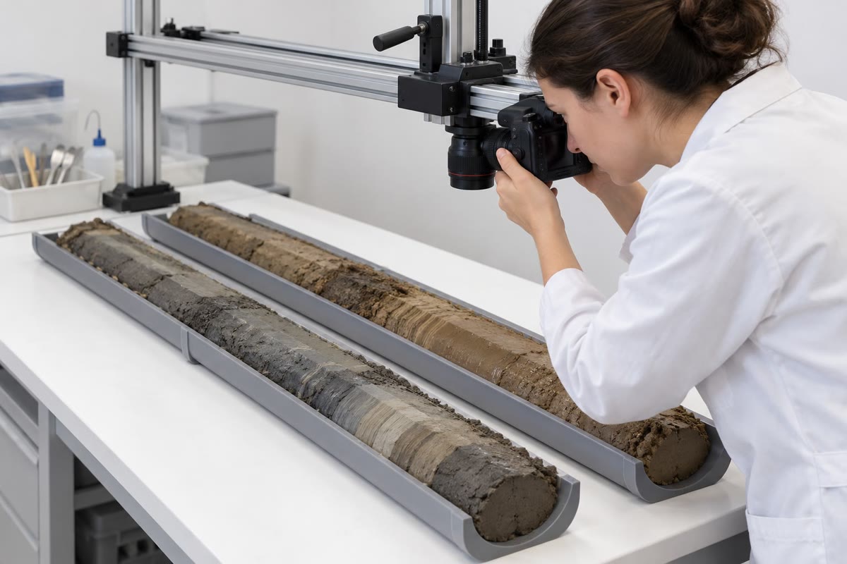
The cylinders of sediment or rock brought up by a drill are laid in trays in the order of depth, split lengthwise, and photographed under even light before they dry and change colour. The sedimentologist then draws a log of the core, metre by metre: the lithology, the grain size of each bed (the width of the column), the structures (cross-bedding, lamination, grading, burrows), the contacts, sharp or gradual, the colour and the fossils. Samples are taken for grain-size analysis and thin sections. A core is a single narrow window: the direction of the cross-beds is lost unless the core was oriented, and the lateral extent of the beds must come from other boreholes.

21.4 Shoreline and shelf

Along the coast between the deltas, the sand brought by the rivers is shaped by waves and tides. A beach is sand reworked by the swash, the thin sheet of water that runs up and down it after each wave breaks: the grains are moved again and again, the fine ones are carried offshore, and beach sands are among the best sorted and most rounded of all sediments. Their laminae, laid down by the swash, dip gently seaward. On many low coasts the sand forms barrier islands, long ridges of beach and wind-blown dunes separated from the mainland by lagoons, which are quiet and fine-grained, connected to the sea by tidal inlets.

Where the tides are strong and the waves weak, the coast is fringed by tidal flats, covered and uncovered twice a day. They grade from sand near the low-tide line, where the currents are strongest, to mud near the high-tide line, where the slack water lets clay settle; their deposits show the reversing flow in herringbone cross-bedding, the drying in mud cracks, and the alternation of current and slack water in thin draped layers of mud on rippled sand.

Offshore, the shelf is swept by waves only down to a depth that grows with the size of the waves. Above it sand is winnowed and moved; below it mud settles, except during storms, when the larger waves reach deeper and lay down sheets of sand with the gentle undulating lamination called hummocky cross-stratification. A shelf succession thus often alternates fair-weather mud with storm sands, the thicker and coarser toward the shore.

21.5 Deep-sea clastics

Sand and gravel also reach the floors of the deep oceans, thousands of metres down and hundreds of kilometres from land, and they are carried there by flows that no one has seen in full: dense, sediment-laden currents running down the continental slope under the clear water of the ocean.

History — Cables on the sea floor, 1929

On 18 November 1929 an earthquake of moment magnitude 7.2 struck the continental slope south of Newfoundland, along the southern edge of the Grand Banks. A slump of some $200\,\mathrm{km}^{3}$ of sediment moved on the slope, and a tsunami killed 28 people on the coast of Newfoundland. Twelve telegraph cables laid across the sea floor broke, some in several places. Those near the epicentre broke at once; the others, farther south and deeper, broke one after another in the following hours, in order of distance down the slope. In 1952 Bruce Heezen and Maurice Ewing, studying the times of the breaks, explained them: the slump had turned into a turbidity current that ran down the slope and out across the abyssal plain for more than 480 miles, breaking each cable as it passed. From the times and distances they estimated its speed at about 50 knots on the upper continental rise, where the slope is about $0.5\,\%$, and still 12 knots at the last cable, about 400 miles from its origin. As it slowed, they argued, it must have laid down a graded bed over the plain, finer and finer upward.

Fifty knots is $25.7\,\mathrm{m}\,\mathrm{s}^{-1}$, over $90\,\mathrm{km}\,\mathrm{h}^{-1}$, the speed of a car on a main road; 12 knots is $6.2\,\mathrm{m}\,\mathrm{s}^{-1}$; and 480 miles are about $770\,\mathrm{km}$. The breaks also gave the first measured speeds of a flow that had been inferred only from its deposits and from experiments in tanks.

Definition 21.15 (Turbidity current, turbidite, graded bed)

A turbidity current is a current of water made denser than the water around it by the sediment it holds in suspension, which flows down a slope under that water, its grains kept in suspension by the turbulence that its own motion creates. A turbidite is the deposit of a turbidity current. A graded bed is a bed whose grain size decreases from its base to its top.

A turbidity current drives itself: it runs because its suspension is heavy, and it keeps its suspension because it runs. On a steep slope it can pick up more sediment from the bed, become denser and accelerate; on the gentle slope of the abyssal plain it slows, drops its load and dies.

Proposition 21.16 (Speed of a turbidity current)

A turbidity current of thickness $h$ and density $\rho + \Delta\rho$ flows steadily down a slope $S$ under water of density $\rho$. If the resistance of the bed and of the water above is $\tau = \rho\,C_f\,U^2$ per unit area, $C_f$ being a dimensionless friction coefficient, its mean speed is

$$U = \sqrt{\frac{\Delta\rho}{\rho}\,\frac{g\,h\,S}{C_f}} .$$

The resistance law $\tau = \rho C_f U^2$, quadratic in the speed, is the one of turbulent flows in hydraulics (the physics books), and $C_f$ is found by experiment. The formula neglects the water that the current mixes into itself through its upper surface, which dilutes and slows it. It shows the role of the three factors: a current twice as thick, or twice as dense, or on a slope twice as steep, runs $\sqrt 2$ times faster. A suspension holding the fraction $c$ of its volume as quartz grains has $\Delta\rho/\rho = 1.65\,c$ (Section 20.2), small unless the flow is very concentrated; this is where a turbidity current differs from a river, in which the whole weight of the water, not a small excess, drives the flow. To run at the 50 knots of 1929 on a slope of half a per cent, a turbidity current needs a large product of thickness and density excess (Exercise 21.11).

The Bouma sequence. In 1962 Arnold Bouma described the internal order of the sandstone beds of ancient deep-sea successions in five divisions, labelled from the base up. A: massive or graded sand, often on an erosive base; B: sand with parallel lamination; C: fine sand with ripple cross-lamination, often convolute; D: laminated silt grading into mud; E: mud. The order is read as the record of a single waning current passing over a point: as it slows, it drops first its coarsest grains en masse, then builds an upper plane bed, then ripples, then lets the silt and clay settle. Complete sequences are rare: the upper divisions are often eroded by the next current, and far from the source, where the current is weak, the lower ones are missing.

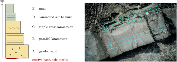
The Bouma sequence became the standard model of the turbidite, and thousands of ancient deep-sea sandstones were interpreted with it. The interpretation is disputed: currents running along the slope, deep tidal currents and internal waves also build rippled and laminated sands, and some sedimentologists argue that many beds read as turbidites, including some of those of the type area, were laid down by other flows. Few turbidity currents have been observed in the modern ocean, while ancient turbidites are counted by the thousands.

Not all deep-sea clastics are turbidites. Contour currents, the slow, deep currents that follow the contours of the continental slope, rework the sediment of the slope into smooth, elongated drifts, the contourites. And far from the continents, where neither turbidity currents nor contour currents reach, the sea floor receives only what settles from the water above: the shells of plankton and the finest windblown dust, the pelagic sediments of the next chapter (Chapter 22).

21.6 Exercises

Exercise 21.1 ★

Convert to phi units the diameters $0.18\,\mathrm{mm}$, $0.75\,\mathrm{mm}$, $3\,\mathrm{mm}$, $0.012\,\mathrm{mm}$ and $150\,\mathrm{mm}$, to two decimals, and name the class of each (Table 21.1).

Solution

Solution of Exercise 21.1.

$\varphi = -\log_2 d$: $0.18\,\mathrm{mm}$ gives $2.47$, a fine sand (2 to 3); $0.75\,\mathrm{mm}$ gives $0.42$, a coarse sand (0 to 1); $3\,\mathrm{mm}$ gives $-1.58$, a granule ($-1$ to $-2$); $0.012\,\mathrm{mm}$ gives $6.38$, a fine silt (6 to 7); $150\,\mathrm{mm}$ gives $-7.23$, a cobble ($-6$ to $-8$).

Exercise 21.2 ★

The cumulative curve of a river sand gives $\varphi_5 = 0.62$, $\varphi_{16} = 1.05$, $\varphi_{50} = 1.71$, $\varphi_{84} = 2.43$ and $\varphi_{95} = 2.98$. Compute its graphic mean, in phi units and in millimetres, and its inclusive graphic standard deviation, and name its size and its sorting.

Solution

Solution of Exercise 21.2.

$M_z = (1.05 + 1.71 + 2.43)/3 = 1.73\,\varphi$, that is $2^{-1.73} = 0.30\,\mathrm{mm}$, a medium sand. $\sigma_I = (2.43 - 1.05)/4 + (2.98 - 0.62)/6.6 = 0.345 + 0.358 = 0.70\,\varphi$: moderately well sorted (0.50 to 0.71), just below the limit of moderately sorted.

Exercise 21.3 ★

Ripples $2\,\mathrm{cm}$ high migrate at $1\,\mathrm{cm}$ a minute over a bed of quartz sand of porosity $0.4$. With Proposition 21.7, compute the volume of bed load per unit width, in $\mathrm{m}^{2}\,\mathrm{s}^{-1}$, and the mass of quartz ($2650\,\mathrm{kg}\,\mathrm{m}^{-3}$) carried over a metre of crest in a day.

Solution

Solution of Exercise 21.3.

$q_b = (1 - 0.4) \times 0.02 \times (0.01/60)/2 = 1.0 \times 10^{-6}\,\mathrm{m}^{2}\,\mathrm{s}^{-1}$ of solid grains. In a day, $1.0 \times 10^{-6} \times 86400 = 0.0864\,\mathrm{m}^{3}$ per metre of crest, or $0.0864 \times 2650 = 229\,\mathrm{kg}$ of quartz.

Exercise 21.4 ★

A knot is one nautical mile, $1852\,\mathrm{m}$, per hour. (a) Convert to metres per second the speeds of 50 and 12 knots estimated for the turbidity current of 1929. (b) How long does a current at 12 knots take to cover $100\,\mathrm{km}$? (c) Convert 480 and 400 miles to kilometres (one mile is $1.609\,\mathrm{km}$).

Solution

Solution of Exercise 21.4.

(a) 50 knots are $50 \times 1852/3600 = 25.7\,\mathrm{m}\,\mathrm{s}^{-1}$; 12 knots, $6.17\,\mathrm{m}\,\mathrm{s}^{-1}$. (b) $100\,000\,\mathrm{m}/6.17\,\mathrm{m}\,\mathrm{s}^{-1} = 16\,200\,\mathrm{s}$, about $4.5\,\mathrm{h}$. (c) 480 miles are $772\,\mathrm{km}$, 400 miles $644\,\mathrm{km}$.

Exercise 21.5 ★★

(a) Using the percentiles of a normal distribution given in the proof of Proposition 21.4, compute the graphic standard deviation $(\varphi_{84} - \varphi_{16})/2$ and the estimate $(\varphi_{95} - \varphi_5)/3.3$ for a normal distribution of standard deviation $\sigma$. (b) Why might the two disagree for a real sediment? Which kind of sediment makes them differ the most?

Solution

Solution of Exercise 21.5.

(a) $(\varphi_{84} - \varphi_{16})/2 = 2 \times 0.9945\,\sigma/2 = 0.9945\,\sigma$, and $(\varphi_{95} - \varphi_5)/3.3 = 2 \times 1.6449\,\sigma/3.3 = 0.9969\,\sigma$: both estimate $\sigma$ to within a third of a per cent. (b) A real sediment need not be normal in phi units: a small admixture of much coarser or much finer grains changes $\varphi_5$ or $\varphi_{95}$ a lot and $\varphi_{16}$ and $\varphi_{84}$ little, so the second estimate grows while the first does not. The two differ most for mixtures, such as a sand with some gravel and mud, or a bimodal deposit.

Exercise 21.6 ★★

A deposit of climbing ripples shows sets $1.5\,\mathrm{cm}$ thick, measured perpendicular to their boundaries, made by ripples spaced at $15\,\mathrm{cm}$. (a) Compute the angle of climb. (b) If the ripples moved at $0.5\,\mathrm{cm}$ a minute, at what rate was the bed raised, in centimetres per hour? (c) What does such a rate say about the flow?

Solution

Solution of Exercise 21.6.

(a) $\sin\theta = T/L = 1.5/15 = 0.1$, so $\theta = 5.74{}^{\circ}$. (b) $a = c\tan\theta = 0.5 \times 0.1005 = 0.050\,\mathrm{cm}$ a minute, or $3.0\,\mathrm{cm}$ an hour. (c) A bed raised by centimetres an hour receives sand falling out of suspension very fast: a heavily loaded current that is slowing down, such as a waning flood or the tail of a turbidity current.

Exercise 21.7 ★★

Six cross-bed dip directions, already corrected for the tilt of the beds, read 350, 020, 005, 340, 015 and 030. (a) Compute their arithmetic mean. (b) Compute their vector mean and $\bar R$. (c) Explain the difference.

Solution

Solution of Exercise 21.7.

(a) $(350 + 20 + 5 + 340 + 15 + 30)/6 = 760/6 = 126.7$: a south-easterly direction, although every reading lies within $20{}^{\circ}$ of north. (b) $S = \sum\sin\alpha_i = 0.672$, $C = \sum\cos\alpha_i = 5.692$, so $\bar\alpha = \operatorname{atan2}(0.672, 5.692) = 6.7{}^{\circ}$, and $\bar R = \sqrt{0.672^2 + 5.692^2}/6 = 5.732/6 = 0.955$. (c) The arithmetic mean treats 350 and 005 as far apart, while on the circle they are $15{}^{\circ}$ apart: azimuths must be averaged as unit vectors. The large $\bar R$ shows that the readings are tightly grouped around $7{}^{\circ}$.

Exercise 21.8 ★★

Three sandstones are examined in thin section. A has $12\,\%$ of clay matrix and angular grains of quartz, feldspar and rock fragments. B has $2\,\%$ of clay, $\sigma_I = 0.40\,\varphi$ and quartz grains of roundness $2.2$ on Folk’s scale. C has no clay, $\sigma_I = 0.30\,\varphi$, quartz grains of roundness $3.6$, and $98\,\%$ quartz. Name the textural maturity of each, and suggest an environment of deposition for each.

Solution

Solution of Exercise 21.8.

A has more than $5\,\%$ of clay: immature, and compositionally immature too, with its feldspar and rock fragments; quickly deposited near its source, on an alluvial fan or a floodplain, or by a turbidity current. B has less than $5\,\%$ clay and is well sorted ($\sigma_I < 0.5\,\varphi$) but its grains are subangular ($\rho < 3$): mature, for example a river bar or a shelf sand winnowed by currents. C has no clay, is very well sorted and its grains are rounded ($\rho > 3$): supermature, and with $98\,\%$ quartz also compositionally mature, as on a beach or in a desert dune field.

Exercise 21.9 ★★

(a) Compute the Froude number of a flow $0.3\,\mathrm{m}$ deep at $1.5\,\mathrm{m}\,\mathrm{s}^{-1}$, and of a river $2\,\mathrm{m}$ deep at $1.0\,\mathrm{m}\,\mathrm{s}^{-1}$ ($g = 9.81\,\mathrm{m}\,\mathrm{s}^{-2}$). (b) At what depth would a flow of $1.5\,\mathrm{m}\,\mathrm{s}^{-1}$ reach a Froude number of 1, and what speed would the river $2\,\mathrm{m}$ deep need? (c) Why are antidunes common in sheets of water running off a beach, and rare in large rivers?

Solution

Solution of Exercise 21.9.

(a) $1.5/\sqrt{9.81 \times 0.3} = 0.87$; $1.0/\sqrt{9.81 \times 2} = 0.23$. (b) $h = U^2/g = 1.5^2/9.81 = 0.23\,\mathrm{m}$; $U = \sqrt{9.81 \times 2} = 4.43\,\mathrm{m}\,\mathrm{s}^{-1}$. (c) The Froude number grows as the depth decreases at a given speed: thin, fast sheets of water, like the backwash of a wave on a beach, easily reach Froude numbers near 1, while a river several metres deep would need several metres per second, which few rivers reach except in floods.

Exercise 21.10 ★★★

A sieve analysis of a sand gives, in whole-phi classes from $-1$ to $5\,\varphi$: 2, 8, 30, 40, 15 and 5 weight per cent. (a) By the method of moments, compute the mean and the standard deviation in phi units, and name the sorting. (b) Build the cumulative curve, read $\varphi_5$, $\varphi_{16}$, $\varphi_{50}$, $\varphi_{84}$ and $\varphi_{95}$ by linear interpolation, and compute $M_z$ and $\sigma_I$. (c) Compare.

Solution

Solution of Exercise 21.10.

(a) With the mid-points $-0.5, 0.5, \ldots, 4.5$: $m = (-1 + 4 + 45 + 100 + 52.5 + 22.5)/100 = 2.23\,\varphi$; the squared deviations weighted by the percentages sum to $107.71$, so $s = \sqrt{1.0771} = 1.04\,\varphi$: poorly sorted. (b) The cumulative per cent coarser is 0, 2, 10, 40, 80, 95 and 100 at $-1, 0, \ldots, 5\,\varphi$. Then $\varphi_5 = 0 + 3/8 = 0.375$, $\varphi_{16} = 1 + 6/30 = 1.20$, $\varphi_{50} = 2 + 10/40 = 2.25$, $\varphi_{84} = 3 + 4/15 = 3.27$, $\varphi_{95} = 4.0$. $M_z = (1.20 + 2.25 + 3.27)/3 = 2.24\,\varphi$ and $\sigma_I = (3.27 - 1.20)/4 + (4.0 - 0.375)/6.6 = 0.517 + 0.549 = 1.07\,\varphi$. (c) The two methods agree to about $0.01$ on the mean and $0.03$ on the sorting: a fine sand ($2.24\,\varphi$ is $0.21\,\mathrm{mm}$), poorly sorted.

Exercise 21.11 ★★★

Take $C_f = 0.003$ in Proposition 21.16. (a) A turbidity current $50\,\mathrm{m}$ thick, with a density excess of $2\,\%$, runs down a slope of $0.005$: compute its speed, in metres per second and in knots. (b) What product of thickness and relative density excess would give the 50 knots of 1929 on the same slope? (c) The same current as in (a) reaches a slope of $0.001$: compute its new speed, if nothing else changes. What happens to its load?

Solution

Solution of Exercise 21.11.

(a) $U = \sqrt{0.02 \times 9.81 \times 50 \times 0.005/0.003} = 4.04\,\mathrm{m}\,\mathrm{s}^{-1}$, or 7.9 knots. (b) $(\Delta\rho/\rho)\,h = U^2 C_f/(gS) = 25.7^2 \times 0.003/(9.81 \times 0.005) = 40\,\mathrm{m}$: for instance a current $400\,\mathrm{m}$ thick with a density excess of $10\,\%$, which shows how large and dense the current of 1929 must have been. (c) The speed scales as $\sqrt S$: $4.04/\sqrt 5 = 1.81\,\mathrm{m}\,\mathrm{s}^{-1}$. The slower current has weaker turbulence and drops its coarser grains; it becomes less dense, slows further, and spreads its load over the plain as a graded bed.

Exercise 21.12 ★★★

A river delivers $50\,\mathrm{Mt}$ of sediment a year to its delta, of which $70\,\%$ is deposited on a delta front $100\,\mathrm{km}$ wide that builds into water $30\,\mathrm{m}$ deep. The deposit has a bulk density of $2000\,\mathrm{kg}\,\mathrm{m}^{-3}$. (a) What volume does it add each year? (b) If this volume fills the whole depth of water along the width of the front, how fast does the front advance? (c) With a delta-front slope of $0.5{}^{\circ}$, at what rate does sediment pile up at a fixed point under the front, and in how many years does the coarsening-upward succession form there?

Solution

Solution of Exercise 21.12.

(a) $0.7 \times 5 \times 10^{10}\,\mathrm{kg}/2000\,\mathrm{kg}\,\mathrm{m}^{-3} = 1.75 \times 10^{7}\,\mathrm{m}^{3}$ a year. (b) Spread over a front $30\,\mathrm{m}$ high and $100\,\mathrm{km}$ wide, it advances the front by $1.75 \times 10^{7}/(30 \times 1 \times 10^{5}) = 5.8\,\mathrm{m}$ a year. (c) $a = v\tan\alpha = 5.83 \times \tan0.5{}^{\circ} = 0.051\,\mathrm{m}$, about $5\,\mathrm{cm}$ a year, a hundred times less than the advance; the $30\,\mathrm{m}$ succession forms in $30/0.051 = 590$ years.

21.7 Problem: Reading a core from a delta

Problem 21.1

Weekend problem — a borehole through an ancient delta, from the grain sizes to the direction of its rivers

A borehole crosses $24\,\mathrm{m}$ of sandstones and mudstones laid down by an ancient delta. The geologist describes four units, from the base up, and analyses a sample of each.

unit (depth from the base)	description	$\varphi_5$	$\varphi_{16}$	$\varphi_{50}$	$\varphi_{84}$	$\varphi_{95}$
1 (0–8 m)	laminated grey mudstone	4.2	5.0	6.6	8.4	9.6
2 (8–16 m)	alternating siltstone and sandstone	1.9	2.4	3.4	4.6	5.5
3 (16–21 m)	cross-bedded sandstone	0.9	1.25	1.8	2.35	2.7
4 (21–24 m)	pebbly sandstone, erosive base	$-1.8$	$-0.8$	0.9	2.1	2.9

Part I — The grain sizes.

1. Compute the graphic mean $M_z$ of each unit, in phi units and in millimetres.
2. Compute the inclusive graphic standard deviation $\sigma_I$ of each unit.
3. Name the size class of the mean and the sorting of each unit.
4. Which unit is the best sorted? Why would a mouth bar be better sorted than the prodelta muds?
5. Interpolating linearly between $\varphi_{50}$ and $\varphi_{84}$, estimate the percentage of clay-sized particles (finer than $8\,\varphi$) in unit 1. What does it say about the currents where it was deposited?
6. Why is the cumulative curve of unit 4 so spread out, although it is a channel sand?

Part II — The succession.

7. Describe how the mean size changes from unit 1 to unit 3. Is the succession fining or coarsening upward?
8. Interpret units 1, 2 and 3 as parts of a delta. Which zone of the delta was at the site when each was deposited?
9. What does the stacking of the three units show about the movement of the delta?
10. What depth of water did the delta build into, at least, and why?
11. Unit 4 has an erosive base and is coarser than unit 3. Interpret it.
12. Would a point bar give the same succession? Explain.

Part III — How fast did the delta advance? Two thin beds of volcanic ash, at the base of unit 1 and at the top of unit 2, are dated; they are $4000$ years apart.

13. Compute the mean rate of accumulation between the two ashes, in millimetres a year.
14. The delta front sloped at $0.5{}^{\circ}$. With Proposition 21.14, compute the speed at which it advanced, in metres a year.
15. How far did the front advance during the $4000$ years?
16. How long did the 21 metres of units 1 to 3 take to accumulate at the site, at this rate?
17. Why is the rate of accumulation in a delta not the same everywhere at the same time?

Part IV — Where did the rivers flow? On the cross-bedded sandstone of unit 3, exposed in a nearby outcrop where the beds are horizontal, twelve foreset dip directions are measured: 352, 010, 025, 004, 338, 017, 031, 359, 012, 046, 006 and 344.

18. Compute the arithmetic mean of the twelve readings. Is it meaningful?
19. Compute the sums $S$ and $C$ of Proposition 21.10.
20. Compute the mean resultant length $\bar R$. Are the readings consistent?
21. In which general direction did the delta build, and where was the land?
22. Why must the dip directions be rotated if the beds are tilted, and about which axis?
23. Could a tidal current have built these cross-beds? What would its rose diagram look like?
24. To the nearest degree, what is the mean palaeocurrent azimuth of the cross-bedded sandstone of unit 3?

Solution

Solution of Problem 21.1.

1. Unit 1: $(5.0 + 6.6 + 8.4)/3 = 6.67\,\varphi$, $0.0098\,\mathrm{mm}$ ($9.8\,\text{µ}\mathrm{m}$); unit 2: $3.47\,\varphi$, $0.090\,\mathrm{mm}$; unit 3: $1.80\,\varphi$, $0.29\,\mathrm{mm}$; unit 4: $0.73\,\varphi$, $0.60\,\mathrm{mm}$.

2. Unit 1: $(8.4 - 5.0)/4 + (9.6 - 4.2)/6.6 = 0.850 + 0.818 = 1.67\,\varphi$; unit 2: $0.550 + 0.545 = 1.10$; unit 3: $0.275 + 0.273 = 0.55$; unit 4: $0.725 + 0.712 = 1.44$.

3. Unit 1: fine silt, poorly sorted; unit 2: very fine sand, poorly sorted; unit 3: medium sand, moderately well sorted; unit 4: coarse sand, poorly sorted.

4. Unit 3. At the river mouth the current and the waves move the sand again and again and carry the fines away, while the prodelta mud settles from suspension as a mixture of all the fine sizes that reach it.

5. The size $8\,\varphi$ lies $1.4/1.8$ of the way from $\varphi_{50}$ to $\varphi_{84}$, so $50 + (1.4/1.8) \times 34 = 76$ per cent of the sample is coarser and about $24\,\%$ is clay-sized. Such fine particles settle only from nearly still water: the site was below the reach of waves and currents.

6. A channel carries both gravel, rolled on its bed in floods, and sand; the deposit mixes the gravel lag of the deepest flow with the sand of lower flows, so it covers many classes.

7. The mean grows from $0.0098\,\mathrm{mm}$ to $0.090\,\mathrm{mm}$ and $0.29\,\mathrm{mm}$: the succession coarsens upward.

8. Unit 1, laminated mud: the prodelta; unit 2, alternating silt and sand: the lower delta front; unit 3, cross-bedded sand: the mouth bars of the upper delta front.

9. Each zone came to lie on the one that was formerly in front of it: the delta built forward, seaward, over the site.

10. At least $21\,\mathrm{m}$, the thickness of units 1 to 3, since the succession filled the water from the floor of the prodelta to the mouth bar near the surface; more, since the muds have been compacted since (Chapter 23).

11. A distributary channel of the delta plain, cutting into the mouth bar as the delta built forward; its pebbles are its bed load.

12. No: a point bar starts with an erosion surface and a lag and fines upward, to floodplain mud. The delta front coarsens upward from mud.

13. $16\,\mathrm{m}/4000\text{ years} = 4.0\,\mathrm{mm}$ a year.

14. $v = a/\tan\alpha = 0.0040/\tan0.5{}^{\circ} = 0.0040/0.008727 = 0.458\,\mathrm{m}$ a year.

15. $0.458 \times 4000 = 1830\,\mathrm{m}$, about $1.8\,\mathrm{km}$.

16. $21\,\mathrm{m}/4.0\,\mathrm{mm}\,\mathrm{yr}^{-1} = 5250$ years.

17. The delta front receives most of the sand near the mouths, the prodelta far less and the delta plain little except in floods; the active mouths also shift from place to place, so a point may receive much for a while and then almost nothing. A single rate between two dated beds is an average over these changes, and the muds have lost part of their thickness by compaction.

18. The sum is 1544, so the arithmetic mean is $128.7{}^{\circ}$, a south-easterly direction: meaningless, since the readings scatter around north and the values near 340 and near 010 are averaged as if they were far apart.

19. $S = \sum\sin\alpha_i = 1.698$ and $C = \sum\cos\alpha_i = 11.248$.

20. $\bar R = \sqrt{1.698^2 + 11.248^2}/12 = 11.376/12 = 0.948$: the readings are tightly grouped around one direction.

21. The rivers flowed, and the delta built, toward about north (Proposition 21.10); the land lay to the south.

22. Because the foresets were measured on beds that are no longer horizontal: their dip directions are those of the tilted beds plus the tilting. Rotating each foreset about the strike of the bedding by the dip of the bedding restores the bedding, and with it the foresets, to their original attitude.

23. Tidal currents flow in and out, and build sets that dip in two opposite directions, as in herringbone cross-bedding; the rose diagram would have two lobes about $180{}^{\circ}$ apart. The twelve readings form one lobe, $\bar R$ near 1: a river current flowing one way.

24. $\bar\alpha = \operatorname{atan2}(1.698, 11.248) = 8.6{}^{\circ}$: the mean palaeocurrent azimuth of unit 3 is $9{}^{\circ}$, a little east of north.