11Isostasy and Gravity Anomalies

In the 1840s the surveyors measuring a meridian arc across northern India met a discrepancy they could not blame on their instruments. Between two stations about 370 miles apart, Kaliana near the foot of the Himalaya and Kalianpur far to the south, the difference of latitude found by triangulation exceeded the difference found from the stars by 5.236 seconds of arc. The obvious culprit was the mountains: their attraction pulls a plumb line northwards, and the astronomers set their instruments by the plumb line. In 1855 John Henry Pratt computed the attraction of the Himalaya and of the plateaux beyond them and found that it should have made the discrepancy 15.885 seconds, more than three times what was observed. The mountains pulled much less than their visible mass required. The same year George Airy answered that the crust floats on a denser layer like a raft of logs on water, so that high ground has a deep root of light rock; Pratt later proposed another answer, rock made lighter by expansion beneath the mountains. Both are still taught: the mountains are underlain by light rock that makes up for their mass. This chapter turns that idea into numbers, and shows how gravity, measured to a millionth of its value, reveals the masses hidden below the relief.

You already know

Newton’s law of gravitation gives the field $g = GM/r^2$ outside a spherical mass $M$; the field derives from a gravitational potential, and an equipotential surface is everywhere perpendicular to the field (physics). In a fluid at rest the pressure increases with depth as $\mathrm dp/\mathrm dz = \rho g$, and a floating body displaces its own weight of fluid (physics, University Year 1). Below the lithosphere the asthenosphere flows over long times; the crust is lighter than the mantle below it (Chapter 9; Book 2, grade 11).

11.1 Gravity and its measurement

The acceleration of gravity at the Earth’s surface is close to $9.8\,\mathrm{m}\,\mathrm{s}^{-2}$, and the variations that interest geologists are a million times smaller. They are counted in a unit of the old centimetre–gram system, the gal: $1\,\mathrm{Gal} = 1\,\mathrm{cm}\,\mathrm{s}^{-2} = 0.01\,\mathrm{m}\,\mathrm{s}^{-2}$, so that

A field instrument resolves a few thousandths of a milligal; the anomalies studied in this chapter range from a fraction of a milligal over a buried ore body to a few hundred milligals over a mountain range.

Even on a featureless Earth, gravity would not be the same everywhere. The Earth turns, so that what a plumb line or a gravimeter feels is the sum of the gravitational attraction and the centrifugal effect of rotation; and the Earth is flattened, so that the poles are nearer its centre than the equator. Both effects make gravity weaker at the equator than at the poles. A geologist compares every measurement with a smooth reference that contains them.

Definition 11.1 (Normal gravity)

Normal gravity $\gamma$ is the gravity of a model Earth: an ellipsoid of revolution with the Earth’s mass and rotation, chosen so that its surface is an equipotential of its own gravity (gravitation plus the centrifugal effect). On that surface, normal gravity depends on latitude alone.

The ellipsoid itself, its flattening and the way its parameters are fitted to the real Earth are studied in Book 5. Here we only need its gravity.

Proposition 11.2 (The normal gravity formula)

On the reference ellipsoid adopted in 1980, normal gravity at the geographic latitude $\varphi$ is, in its usual series form,

$$\gamma(\varphi) = 9.780\,327\,\mathrm{m}\,\mathrm{s}^{-2}\,\bigl(1 + 0.0053024\sin^2\varphi - 0.0000058\sin^2 2\varphi\bigr).$$

It gives $9.780\,327\,\mathrm{m}\,\mathrm{s}^{-2}$ at the equator, $9.806\,200\,\mathrm{m}\,\mathrm{s}^{-2}$ at $45{}^{\circ}$ and $9.832\,186\,\mathrm{m}\,\mathrm{s}^{-2}$ at the poles: a difference of $5186\,\mathrm{m}\mathrm{Gal}$ from equator to pole. The rotation alone accounts for most of it. With the sidereal day of $23.9345\,\mathrm{h}$, the angular velocity is $\omega = 2\pi/86\,164\,\mathrm{s} = 7.292 \times 10^{-5}\,\mathrm{rad}\,\mathrm{s}^{-1}$, and the centrifugal acceleration at the equator, $\omega^2 a$ with $a = 6378.137\,\mathrm{km}$, is $0.0339\,\mathrm{m}\,\mathrm{s}^{-2}$, or $3392\,\mathrm{m}\mathrm{Gal}$; the flattening supplies the rest (Exercise 11.2).

Gravity is measured in two ways. An absolute gravimeter drops a test mass in a vacuum chamber and follows its free fall with a laser interferometer, timed by an atomic clock: the acceleration comes out directly from distance and time. A relative gravimeter is a mass hung on a spring, whose stretch changes with gravity; it is light and fast, but it only gives differences between places, and it drifts, so a survey returns to a base station whose gravity is known. The best absolute instruments are accurate to about a microgal, a part in a billion of $g$.

In the field — A gravity survey on land

A gravity survey is a slow walk from station to station. At each one the geophysicist sets the relative gravimeter on its tripod, levels it, waits for the spring to settle and takes several readings; a satellite-positioning receiver beside it records the station’s position and height. Every few hours the team goes back to the base station, so that the drift of the spring can be measured and removed. The height matters as much as the gravity: as the next section shows, gravity falls by $0.3086\,\mathrm{m}\mathrm{Gal}$ for every metre of height, so a height wrong by $1\,\mathrm{cm}$ spoils the reading by $3\,\text{µ}\mathrm{Gal}$.

11.2 Isostasy

The compensation that Airy and Pratt imagined for the Himalaya is an instance of a general state of the Earth’s outer layers.

Definition 11.3 (Isostasy; compensation depth)

A region is in isostasy, or isostatic equilibrium, when there exists a depth, the compensation depth, at which the pressure is the same at every point of the horizontal surface, whatever the relief above. Below the compensation depth the rocks behave as a fluid at rest; above it, the columns of crust and mantle float on them.

Proposition 11.4 (Equal masses above the compensation depth)

If gravity $g$ is the same along all the columns, a region is in isostasy with compensation depth $z_c$ if and only if every vertical column of unit cross-section, from the surface down to $z_c$, contains the same mass.

Two simple ways of distributing the masses give the two classical models (figure below).

Proposition 11.5 (Airy isostasy)

Let the crust have a uniform density $\rho_c$ and a thickness $H$ where its surface is at sea level, over a mantle of density $\rho_m > \rho_c$. In isostatic equilibrium:

1. where the surface stands at a height $h$ above sea level, the crust has a root of depth $r = h\,\rho_c/(\rho_m - \rho_c)$ below the normal crust, and a thickness $H + h + r$;
2. where the surface lies at a depth $d$ below sea level, under water of density $\rho_w$, the crust has an anti-root: its base is raised by $r' = d\,(\rho_c - \rho_w)/(\rho_m - \rho_c)$, and its thickness is $H - d - r'$.

This is Airy isostasy: compensation by changes of thickness at constant density.

Proposition 11.6 (Pratt isostasy)

Let every column end at the same compensation depth $D$ below sea level, with a uniform density in each column, $\rho_0$ where the surface is at sea level. In isostatic equilibrium a column whose surface stands at a height $h$ has the density

$$\rho(h) = \rho_0\,\frac{D}{D + h},$$

and a column under a depth $d$ of water has the density $\rho = (\rho_0 D - \rho_w d)/(D - d)$. This is Pratt isostasy: compensation by changes of density at constant depth.

With $\rho_c = 2700\,\mathrm{kg}\,\mathrm{m}^{-3}$ and $\rho_m = 3300\,\mathrm{kg}\,\mathrm{m}^{-3}$, Airy’s root is $h\times2700/600 = 4.5\,h$: a range $2\,\mathrm{km}$ high has a root of $9\,\mathrm{km}$, a plateau $4\,\mathrm{km}$ high one of $18\,\mathrm{km}$. In Pratt’s model with $D = 100\,\mathrm{km}$ and $\rho_0 = 2700\,\mathrm{kg}\,\mathrm{m}^{-3}$, the same two columns have the densities 2647 and $2596\,\mathrm{kg}\,\mathrm{m}^{-3}$, two and four per cent lighter. Both models balance the same masses; they differ in where the light rock sits, and that is something seismology can see: Airy predicts a Moho that deepens under the mountains, Pratt a flat one.

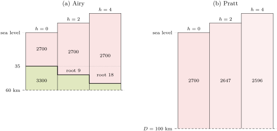
Isostasy is a statement about wide regions over long times. The asthenosphere yields only to loads that persist for thousands of years, and the lithosphere above it is stiff enough to spread a narrow load over a broad region by bending, as a plank carries a weight: a single volcano need not be compensated beneath itself; this flexure of the lithosphere is studied in Book 5. Under large mountain ranges the crust is far thicker than its continental average of about $30\,\mathrm{km}$: Airy’s picture, roots of light crust, is the closer one for mountain ranges. Pratt’s, lighter rock at constant depth, explains the mid-ocean ridges, which stand high over an upper mantle made lighter by its higher temperature.

The Earth’s two levels

Isostasy organises the relief of the whole planet. Its distribution is summarised by one curve.

Definition 11.7 (Hypsometric curve)

The hypsometric curve of a planet gives, for each fraction $f$ of its surface, the elevation $z(f)$ exceeded by exactly that fraction. It is the cumulative distribution of elevation, read from the top.

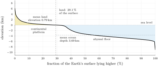
To draw it from a gridded elevation model, every grid cell must be weighted by its area. On a grid of one degree in latitude and longitude, the cell between the latitudes $\varphi_1$ and $\varphi_2$ has the area $R^2\,\Delta\lambda\,(\sin\varphi_2 - \sin\varphi_1)$, which shrinks towards the poles; summed over all cells, the areas give $4\pi R^2$ exactly. Sorting the cells by elevation and accumulating their areas gives the curve of the figure below. It shows that $70.9\,\%$ of the surface lies below sea level; that the mean elevation of the land is about $0.8\,\mathrm{km}$ and the mean depth of the ocean about $3.7\,\mathrm{km}$; and that most of the surface belongs to one of two flat steps, the continental platforms near sea level and the abyssal floor between about 3.5 and $6\,\mathrm{km}$ down, joined by a steep drop.

A planet with a single kind of crust, its relief raised and worn at random, would have one level, with elevations scattered around it. The Earth has two, because it has two kinds of crust in isostatic equilibrium: the thick, light continental crust floats high, the thin, dense oceanic crust low (Book 2, grade 11). Exercise 11.8 shows that Airy’s model with one crustal density cannot produce both levels with the observed crustal thicknesses.

11.3 Gravity anomalies

Two corrections

A gravimeter on a hill is farther from the Earth’s centre than one at sea level, and stands on a layer of rock that the other does not have. Both effects are computed before the measurement is compared with normal gravity.

Proposition 11.8 (Free-air gradient)

Outside a spherical Earth of radius $R$, gravity decreases with height $h$ at the rate

$$\frac{\mathrm dg}{\mathrm dh} = -\frac{2g}{R}\,;$$

at the surface, $2g/R \approx 3.08 \times 10^{-6}\,\mathrm{s}^{-2}$, about $0.308\,\mathrm{m}\mathrm{Gal}$ per metre.

The flattening and the rotation change the gradient slightly; the value used in practice is $0.3086\,\mathrm{m}\mathrm{Gal}\,\mathrm{m}^{-1}$.

Proposition 11.9 (Bouguer slab)

An infinite horizontal slab of thickness $h$ and uniform density $\rho$ attracts a point outside it with the vertical acceleration

$$g_B = 2\pi G\rho h ,$$

whatever the distance from the point to the slab. Numerically $2\pi G = 0.0419\,\mathrm{m}\mathrm{Gal}$ per metre of thickness per $1000\,\mathrm{kg}\,\mathrm{m}^{-3}$ of density.

Definition 11.10 (Gravity anomalies)

Let $g$ be the gravity measured at a station of latitude $\varphi$ and height $h$ above sea level.

• A gravity anomaly is the difference between the measured gravity, corrected to a common level, and the normal gravity at the same latitude.
• The free-air correction is $+0.3086\,\mathrm{m}\mathrm{Gal}\,\mathrm{m}^{-1}\times h$: it adds back the decrease of gravity with height. The free-air anomaly is $\Delta g_{\mathrm{FA}} = g + 0.3086\,h - \gamma(\varphi)$.
• The Bouguer correction is $-2\pi G\rho h$: it removes the attraction of the rock between the station and sea level, treated as a slab of density $\rho$, conventionally $2670\,\mathrm{kg}\,\mathrm{m}^{-3}$, which gives $0.112\,\mathrm{m}\mathrm{Gal}$ per metre. The Bouguer anomaly is $\Delta g_{\mathrm B} = \Delta g_{\mathrm{FA}} - 2\pi G\rho h$.

The slab is a crude model of the ground around a station in rough country: valleys below the station are counted as rock that is not there, hills above it pull upwards and are not counted at all. A third reduction, the terrain correction, computed from a digital elevation model, removes both errors. At sea the free-air correction vanishes, and the Bouguer reduction replaces the water by rock.

Method 11.11 (Reducing a gravity reading)

1. Compute the normal gravity $\gamma(\varphi)$ at the station’s latitude.
2. Add the free-air correction $0.3086\,h$ (in $\mathrm{m}\mathrm{Gal}$, with $h$ in metres) to the measured gravity and subtract $\gamma$: this is the free-air anomaly.
3. Subtract the Bouguer correction $0.0419\times(\rho/1000)\times h$, that is $0.112\,h$ for the standard density: this is the Bouguer anomaly.
4. Work in milligals throughout, and keep the measured and normal gravity to seven significant figures: the anomaly is a small difference of two large numbers.

Example 11.12 (A station in the hills)

At a station at latitude $45{}^{\circ}$ and $1200\,\mathrm{m}$ above sea level, the gravimeter gives $9.802\,597\,\mathrm{m}\,\mathrm{s}^{-2}$. Normal gravity there is $9.806\,200\,\mathrm{m}\,\mathrm{s}^{-2}$; the measured value is lower by $360.3\,\mathrm{m}\mathrm{Gal}$. The free-air correction is $0.3086\times1200 = 370.3\,\mathrm{m}\mathrm{Gal}$, so $\Delta g_{\mathrm{FA}} = -360.3 + 370.3 = +10.0\,\mathrm{m}\mathrm{Gal}$. The Bouguer correction is $0.112\times1200 = 134.4\,\mathrm{m}\mathrm{Gal}$, so $\Delta g_{\mathrm B} = -124.4\,\mathrm{m}\mathrm{Gal}$: there is less mass below this station than below a station at sea level, once the rock above sea level is removed.

What the anomalies say about compensation

Proposition 11.13 (Anomalies over broad relief)

Consider a plateau of height $h$ and density $\rho_c$, much wider than its compensation depth, and a station near its centre. Take the Bouguer density equal to $\rho_c$.

1. If the plateau is not compensated, $\Delta g_{\mathrm{FA}} \approx 2\pi G\rho_c h$ and $\Delta g_{\mathrm B} \approx 0$.
2. If it is in isostatic equilibrium, whatever the distribution of the compensating masses, $\Delta g_{\mathrm{FA}} \approx 0$ and $\Delta g_{\mathrm B} \approx -2\pi G\rho_c h$.

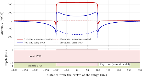
For Airy compensation the Bouguer anomaly of the second case is also $-2\pi G(\rho_m - \rho_c)r$, the attraction of the missing mass of the root, since $(\rho_m - \rho_c)r = \rho_c h$. Free-air anomalies near zero over wide regions are thus the signature of isostasy, and Bouguer anomalies that follow the relief in mirror image measure the compensating masses: the Bouguer anomalies are regionally negative all along the Alps, and over the mid-ocean ridges, high as they are, the free-air anomaly is small. Over the oceans the Bouguer anomaly is positive: replacing the water by rock adds mass above a column that has none missing.

Near the edges of the relief the slab approximation fails, because the topography is close to the station and the root far below it. The figure below gives the exact attraction of a model range $200\,\mathrm{km}$ wide and $2\,\mathrm{km}$ high. Without compensation, the free-air anomaly is $+225\,\mathrm{m}\mathrm{Gal}$ at the centre, close to the slab value of $226\,\mathrm{m}\mathrm{Gal}$; with an Airy root of $9\,\mathrm{km}$, the centre free-air anomaly falls to $+55\,\mathrm{m}\mathrm{Gal}$, not zero, because a range only $200\,\mathrm{km}$ wide does not look infinite from $40\,\mathrm{km}$ above its root, and the free-air anomaly turns sharply negative just beyond each edge, where the station sees the root but not the mountain.

Method 11.14 (Testing a region for isostasy)

1. Average the free-air anomaly over an area several times wider than the crust is thick, away from the edges of the relief.
2. If it is near zero, the region is compensated; if it approaches $2\pi G\rho_c$ times the mean height, it is not.
3. The ratio $-\Delta g_{\mathrm B}/(2\pi G\rho_c h)$ gives the fraction of the relief that is compensated.
4. Seismic or other evidence on the depth of the Moho tells Airy’s compensation from Pratt’s: broad gravity alone cannot, since both put the same mass deficit below the relief.

History — Gravity at sea

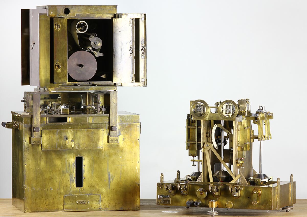
A pendulum measures gravity through its period, but on a ship the waves shake it far more than any anomaly. In the 1920s the Dutch geodesist Felix Vening Meinesz found the way round: two pendulums swinging in opposite phase in the same frame feel the same horizontal accelerations of the ship, and their difference cancels them. From 1923 he carried his apparatus on submarines of the Dutch navy, where, submerged, it was spared the worst of the waves, first on a voyage to the East Indies and then in surveys of their seas. Along the deep-sea trenches of the archipelago he found long belts of strongly negative isostatic anomalies, and then found them along other trenches: he could explain them only by a crust held down there by outside forces, out of isostatic equilibrium.

11.4 The geoid

The sea surface at rest is a surface of constant gravity potential: if it were not, water would flow along it. It is the natural reference for heights, and the surface the old plumb lines were perpendicular to.

Definition 11.15 (Geoid; geoid height)

The geoid is the equipotential surface of the Earth’s gravity (gravitation plus the centrifugal effect of rotation) that coincides with the mean sea surface over the open oceans, at rest, and is continued beneath the continents. The geoid height $N$ at a point is the height of the geoid above the reference ellipsoid, counted negative where the geoid lies below it.

Heights above sea level on maps are heights above the geoid; the heights given by satellite positioning are heights above the ellipsoid; the two differ by $N$. The geoid departs from the ellipsoid by $+85\,\mathrm{m}$ near Iceland and $-106\,\mathrm{m}$ off southern India, less than $200\,\mathrm{m}$ in all, while the relief of the solid surface spans about $20\,\mathrm{km}$: the geoid is a far smoother surface than the ground.

Proposition 11.16 (Geoid height and potential anomaly)

Let $\Phi$ be the Earth’s gravity potential and $\Phi_n$ the normal potential, that of the model Earth whose surface, the reference ellipsoid, has the same potential $\Phi_0$ as the geoid, both counted with the sign of physics (the potential increases upwards and $g = -\nabla\Phi$). Let $T = \Phi - \Phi_n$ be the potential anomaly at the geoid. To first order,

$$N = -\frac{T}{\gamma} .$$

Geodesists, who count the potential with the opposite sign, write the same result $N = T/\gamma$, Bruns’ formula.

An excess of mass below a point makes the potential there more negative, so $T < 0$ and $N > 0$: the geoid bulges up over excess mass and sinks over a deficit. The $85\,\mathrm{m}$ of the high near Iceland correspond to a potential anomaly of $-85\,\mathrm{m}\times9.8\,\mathrm{m}\,\mathrm{s}^{-2} \approx -830\,\mathrm{J}\,\mathrm{kg}^{-1}$. Because the potential falls off as $1/r$ while the attraction falls off as $1/r^2$, the geoid is dominated by large, deep masses, and the gravity anomalies by shallow ones. A compensated mountain range raises the geoid only slightly, because its mass excess and its root’s deficit nearly cancel; an uncompensated load raises it much more.

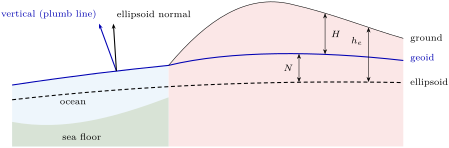
The deflections are small: the whole discrepancy that troubled the surveyors of India was about five seconds of arc. Over the oceans the geoid is visible. Since 1978, radar altimeters on satellites have timed microwave pulses reflected from the sea surface to measure its height. Once tides, waves and currents are averaged away, the sea surface stands higher over seamounts and ridges and lower over trenches and abyssal plains, and these bumps (Exercise 11.11 estimates one) map the topography of the deep ocean floor where no ship has sounded. The satellite GOCE, from 2009 to 2013, flew at about $260\,\mathrm{km}$ and measured the gravity field from orbit, aiming at the geoid to 1 to $2\,\mathrm{cm}$ and the gravity anomalies to about $1\,\mathrm{m}\mathrm{Gal}$, with a resolution better than $100\,\mathrm{km}$.

Isostasy in motion

Isostasy is reached by flow, and flow takes time. At the peak of the last glaciation, about $20\,000$ years ago, an ice sheet about $3\,\mathrm{km}$ thick covered Scandinavia. Ice is about nine tenths as dense as water, so with a mantle of $3300\,\mathrm{kg}\,\mathrm{m}^{-3}$, the full isostatic depression under such a sheet is $3000\,\mathrm{m}\times900/3300 \approx 820\,\mathrm{m}$. The ice has gone, and the land is still rising: satellite positioning measures up to about $10\,\mathrm{mm}\,\mathrm{yr}^{-1}$ of uplift in northern Sweden, west of the Gulf of Bothnia, today. The rate at which a depression relaxes measures the viscosity of the mantle below, the subject of Book 5; Exercise 11.12 shows how.

11.5 Exercises

Exercise 11.1 ★

(a) Convert a Bouguer anomaly of $-150\,\mathrm{m}\mathrm{Gal}$ to $\mathrm{m}\,\mathrm{s}^{-2}$, and express it as a fraction of $g = 9.81\,\mathrm{m}\,\mathrm{s}^{-2}$. (b) The same for $1\,\mathrm{m}\mathrm{Gal}$, the precision aimed at for the gravity anomalies from GOCE, and for $1\,\text{µ}\mathrm{Gal}$.

Solution

Solution of Exercise 11.1.

(a) $-150\,\mathrm{m}\mathrm{Gal} = -150\times10^{-5}\,\mathrm{m}\,\mathrm{s}^{-2} = -1.5 \times 10^{-3}\,\mathrm{m}\,\mathrm{s}^{-2}$, and $1.5 \times 10^{-3}/9.81 = 1.53 \times 10^{-4}$ of $g$. (b) $1\,\mathrm{m}\mathrm{Gal} = 10^{-5}\,\mathrm{m}\,\mathrm{s}^{-2}$, $1.02 \times 10^{-6}$ of $g$; $1\,\text{µ}\mathrm{Gal} = 10^{-8}\,\mathrm{m}\,\mathrm{s}^{-2}$, $1.02 \times 10^{-9}$ of $g$: a gravimeter that resolves a microgal measures gravity to about one part in a billion.

Exercise 11.2 ★

(a) Compute normal gravity at the equator, at $45{}^{\circ}$ and at the poles with the formula of the chapter. (b) Give the equator-to-pole difference in milligals. (c) The centrifugal acceleration at the equator is $3392\,\mathrm{m}\mathrm{Gal}$. What fraction of the difference does the rotation explain directly?

Solution

Solution of Exercise 11.2.

(a) At the equator both sines vanish: $\gamma = 9.780\,327\,\mathrm{m}\,\mathrm{s}^{-2}$. At $45{}^{\circ}$, $\sin^2\varphi = 0.5$ and $\sin^2 2\varphi = 1$: $\gamma = 9.780327\times(1 + 0.0026512 - 0.0000058) = 9.806\,200\,\mathrm{m}\,\mathrm{s}^{-2}$. At the poles, $\sin^2\varphi = 1$ and $\sin 2\varphi = 0$: $\gamma = 9.780327\times1.0053024 = 9.832\,186\,\mathrm{m}\,\mathrm{s}^{-2}$. (b) $9.832186 - 9.780327 = 0.051\,859\,\mathrm{m}\,\mathrm{s}^{-2}$, that is $5186\,\mathrm{m}\mathrm{Gal}$. (c) $3392/5186 = 0.65$: the centrifugal effect explains about two thirds of the difference; the flattening, which puts the poles nearer the centre, the rest.

Exercise 11.3 ★

A plateau stands $3\,\mathrm{km}$ above sea level. With a crust of density $2800\,\mathrm{kg}\,\mathrm{m}^{-3}$ and a mantle of $3300\,\mathrm{kg}\,\mathrm{m}^{-3}$, compute its Airy root and the thickening of its crust.

Solution

Solution of Exercise 11.3.

$r = h\rho_c/(\rho_m - \rho_c) = 3\times2800/500 = 16.8\,\mathrm{km}$. The crust is thicker by $h + r = 19.8\,\mathrm{km}$ (that is $h\rho_m/(\rho_m - \rho_c) = 3\times3300/500$).

Exercise 11.4 ★

(a) By how much must a gravimeter be raised for its reading to fall by $1\,\mathrm{m}\mathrm{Gal}$? Use $0.3086\,\mathrm{m}\mathrm{Gal}\,\mathrm{m}^{-1}$. (b) A survey aims at anomalies to $0.01\,\mathrm{m}\mathrm{Gal}$. To what accuracy must the station heights be known?

Solution

Solution of Exercise 11.4.

(a) $1/0.3086 = 3.24\,\mathrm{m}$. (b) $0.01/0.3086 = 0.032\,\mathrm{m}$: the heights must be known to about $3\,\mathrm{cm}$, which is why a survey records every station’s height with satellite positioning or levelling.

Exercise 11.5 ★★

In Pratt’s model with $D = 100\,\mathrm{km}$ and $\rho_0 = 2700\,\mathrm{kg}\,\mathrm{m}^{-3}$, (a) compute the density of the columns that stand 1, 3 and $5\,\mathrm{km}$ high; (b) compute the density of a column under $4\,\mathrm{km}$ of sea water of density $1030\,\mathrm{kg}\,\mathrm{m}^{-3}$. (c) Why is Pratt’s model better suited to the ocean floor than to the continents?

Solution

Solution of Exercise 11.5.

(a) $\rho = 2700\times100/(100 + h)$: $2673\,\mathrm{kg}\,\mathrm{m}^{-3}$ for $1\,\mathrm{km}$, $2621\,\mathrm{kg}\,\mathrm{m}^{-3}$ for $3\,\mathrm{km}$, $2571\,\mathrm{kg}\,\mathrm{m}^{-3}$ for $5\,\mathrm{km}$. (b) $\rho = (2700\times100 - 1030\times4)/96 = 265\,880/96 = 2770\,\mathrm{kg}\,\mathrm{m}^{-3}$: the column under the sea is denser. (c) Pratt’s model asks for lateral changes of density at a constant depth. Under the ocean floor such changes exist: young, hot lithosphere near a ridge is lighter than old, cold lithosphere far from it (Chapter 10). Under the continents, on the contrary, the thickness of the crust is seen to change with the relief.

Exercise 11.6 ★★

Two stations lie at latitude $48{}^{\circ}$, where normal gravity is $9.808\,911\,\mathrm{m}\,\mathrm{s}^{-2}$. Station 1, $350\,\mathrm{m}$ above sea level, reads $9.807\,751\,\mathrm{m}\,\mathrm{s}^{-2}$; station 2, at $1850\,\mathrm{m}$, reads $9.803\,552\,\mathrm{m}\,\mathrm{s}^{-2}$. (a) Compute the free-air and Bouguer anomalies of both, with the standard Bouguer density. (b) What do the anomalies of station 2 suggest about the mountains around it?

Solution

Solution of Exercise 11.6.

(a) Station 1: $g - \gamma = 9.807751 - 9.808911 = -0.001\,160\,\mathrm{m}\,\mathrm{s}^{-2} = -116.0\,\mathrm{m}\mathrm{Gal}$; free-air correction $0.3086\times350 = 108.0\,\mathrm{m}\mathrm{Gal}$, so $\Delta g_{\mathrm{FA}} = -8.0\,\mathrm{m}\mathrm{Gal}$; Bouguer correction $0.112\times350 = 39.2\,\mathrm{m}\mathrm{Gal}$, so $\Delta g_{\mathrm B} = -47.2\,\mathrm{m}\mathrm{Gal}$. Station 2: $g - \gamma = -535.9\,\mathrm{m}\mathrm{Gal}$; free-air correction $0.3086\times1850 = 570.9\,\mathrm{m}\mathrm{Gal}$, so $\Delta g_{\mathrm{FA}} = +35.0\,\mathrm{m}\mathrm{Gal}$; Bouguer correction $0.112\times1850 = 207.2\,\mathrm{m}\mathrm{Gal}$, so $\Delta g_{\mathrm B} = -172.2\,\mathrm{m}\mathrm{Gal}$. (b) At station 2 the Bouguer anomaly is strongly negative: below the mountains there is a mass deficit, a root of light crust. The free-air anomaly, small compared with the Bouguer correction, shows that the deficit nearly balances the mountains: they are largely compensated (to about $172/207$, or $83\,\%$, if the slab model holds for the whole range).

Exercise 11.7 ★★

(a) Following the proof of Proposition 11.9, show that a horizontal disc of radius $a$, thickness $h$ and density $\rho$ attracts a point on its axis, at a distance $z \gg h$ above it, with $2\pi G\rho h\,\bigl(1 - z/\sqrt{z^2 + a^2}\bigr)$. (b) What radius gives $90\,\%$ of the slab value at $z = 1\,\mathrm{km}$? (c) What does this say about the area of terrain that matters for the Bouguer correction?

Solution

Solution of Exercise 11.7.

(a) As in the proof of the proposition, a thin layer at the distance $z$ contributes $G\rho\,2\pi z\,h\int_0^a s\,(s^2 + z^2)^{-3/2}\,\mathrm ds$, now with the integral stopped at $s = a$: $\int_0^a s\,(s^2 + z^2)^{-3/2}\,\mathrm ds = 1/z - 1/\sqrt{z^2 + a^2}$. Hence $g = 2\pi G\rho h\,\bigl(1 - z/\sqrt{z^2 + a^2}\bigr)$, which tends to the slab value as $a \to \infty$. (b) $z/\sqrt{z^2 + a^2} = 0.1$ gives $\sqrt{z^2 + a^2} = 10z$, $a = \sqrt{99}\,z = 9.95\,\mathrm{km}$ for $z = 1\,\mathrm{km}$. (c) The rock within about ten times its depth below the station supplies $90\,\%$ of the attraction: the terrain correction needs the relief over a radius of several kilometres to tens of kilometres around each station, not only beneath it.

Exercise 11.8 ★★

In Airy’s model with a crust of $2800\,\mathrm{kg}\,\mathrm{m}^{-3}$, $35\,\mathrm{km}$ thick at sea level, over a mantle of $3300\,\mathrm{kg}\,\mathrm{m}^{-3}$, (a) compute the anti-root and the crustal thickness under $4\,\mathrm{km}$ of sea water of density $1030\,\mathrm{kg}\,\mathrm{m}^{-3}$. (b) The oceanic crust is in fact about $5\,\mathrm{km}$ thick. What does the difference show?

Solution

Solution of Exercise 11.8.

(a) $r' = d(\rho_c - \rho_w)/(\rho_m - \rho_c) = 4\times1770/500 = 14.16\,\mathrm{km}$, and the crust is $35 - 4 - 14.16 = 16.84\,\mathrm{km}$ thick. (b) Airy’s model with one crustal density predicts an oceanic crust more than three times too thick. The oceanic crust is not thinned continental crust: it is a different, denser rock, and the two levels of the Earth are two kinds of crust, as the hypsometric curve suggests.

Exercise 11.9 ★★

In the account of the opening, the discrepancy in the difference of latitude between Kaliana and Kalianpur was $5.236''$, while the attraction of the Himalaya computed by Pratt should have produced $15.885''$. (a) Convert both angles to radians. (b) A horizontal acceleration $a_h$ tilts a plumb line by the angle $a_h/g$. What difference of horizontal attraction between the two stations does each angle correspond to, in milligals, with $g = 9.79\,\mathrm{m}\,\mathrm{s}^{-2}$? (c) What fraction of the attraction of the visible mountains did the compensation cancel?

Solution

Solution of Exercise 11.9.

(a) One second of arc is $\pi/(180\times3600) = 1/206\,265$ of a radian: $5.236''$ $= 2.538 \times 10^{-5}\,\mathrm{rad}$ and $15.885''$ $= 7.701 \times 10^{-5}\,\mathrm{rad}$. (b) $a_h = g\theta$: $9.79\times2.538 \times 10^{-5} = 2.485 \times 10^{-4}\,\mathrm{m}\,\mathrm{s}^{-2} = 24.9\,\mathrm{m}\mathrm{Gal}$ observed, and $9.79\times7.701 \times 10^{-5} = 75.4\,\mathrm{m}\mathrm{Gal}$ computed from the visible mountains. (c) $1 - 5.236/15.885 = 0.670$: the compensation cancelled about two thirds of the attraction of the visible mountains.

Exercise 11.10 ★★★

A salt dome is modelled as a sphere of radius $2\,\mathrm{km}$, its centre at $4\,\mathrm{km}$ depth, with a density $200\,\mathrm{kg}\,\mathrm{m}^{-3}$ lower than the rocks around it. (a) Show that a buried sphere of anomalous mass $M$ at depth $z$ gives, at the horizontal distance $x$, the anomaly $GMz/(x^2 + z^2)^{3/2}$. (b) Compute the anomaly above its centre. (c) At what distance has it fallen to half its peak value? (d) How could the depth of a sphere be read from a measured profile?

Solution

Solution of Exercise 11.10.

(a) Outside it, a sphere attracts like a point mass at its centre, with $GM/(x^2 + z^2)$ along the line to the centre; the vertical component is that times the cosine $z/\sqrt{x^2 + z^2}$, which gives $GMz/(x^2 + z^2)^{3/2}$. (b) $M = \tfrac43\pi(2000\,\mathrm{m})^3\times(-200\,\mathrm{kg}\,\mathrm{m}^{-3}) = -6.70 \times 10^{12}\,\mathrm{kg}$, and above the centre $GM/z^2 = 6.674 \times 10^{-11}\times (-6.70 \times 10^{12})/(4000)^2 = -2.80 \times 10^{-5}\,\mathrm{m}\,\mathrm{s}^{-2} = -2.80\,\mathrm{m}\mathrm{Gal}$. (c) $(1 + x^2/z^2)^{-3/2} = 1/2$ gives $x = z\sqrt{2^{2/3} - 1} = 0.766\,z = 3.07\,\mathrm{km}$. (d) The half-width at half-maximum of the profile gives the depth: $z = 1.305\,x_{1/2}$. A deeper body gives a broader, flatter anomaly.

Exercise 11.11 ★★★

A seamount is a cone $3\,\mathrm{km}$ high with a base of radius $15\,\mathrm{km}$ standing on a sea floor $5\,\mathrm{km}$ deep. Its rock has a density of $2800\,\mathrm{kg}\,\mathrm{m}^{-3}$, sea water $1030\,\mathrm{kg}\,\mathrm{m}^{-3}$. (a) Compute its excess mass over the water it displaces. (b) Treat it as a point mass at its centre of mass, a quarter of its height above the base, and use Proposition 11.16 with $\gamma = 9.81\,\mathrm{m}\,\mathrm{s}^{-2}$ to estimate the height of the bump of the sea surface above it. (c) Does the point mass over- or underestimate the bump? (d) If the seamount were fully compensated by a root, how would the bump change?

Solution

Solution of Exercise 11.11.

(a) $V = \tfrac13\pi R^2 H = \tfrac13\pi(15 \times 10^{3}\,\mathrm{m})^2(3 \times 10^{3}\,\mathrm{m}) = 7.07 \times 10^{11}\,\mathrm{m}^{3}$, and $\Delta m = (2800 - 1030)V = 1.25 \times 10^{15}\,\mathrm{kg}$. (b) The centre of mass lies $0.75\,\mathrm{km}$ above the floor, at $d = 5 - 0.75 = 4.25\,\mathrm{km}$ below the sea surface. There the potential anomaly is $T = -G\Delta m/d$, so $N = G\Delta m/(\gamma d) = 6.674 \times 10^{-11}\times1.25 \times 10^{15}/(9.81\times4250) = 2.0\,\mathrm{m}$. (c) Most of the cone’s mass lies in its wide lower part, at 5 to $16\,\mathrm{km}$ from the point above the summit: the mean of $1/r$ over the mass is smaller than $1/4.25\,\mathrm{km}$, and the point mass overestimates the potential. Summing thin discs gives about $1.1\,\mathrm{m}$. (d) A root of light crust beneath would put a deficit of the same mass deeper down; the two potentials nearly cancel, and the bump would be much smaller, but not zero, since the deficit lies farther from the surface than the excess.

Exercise 11.12 ★★★

Model the recovery of Scandinavia after the ice: suppose the ice vanished suddenly $10\,000$ years ago, leaving a depression of $818\,\mathrm{m}$ that has since decreased as $w(t) = w_0\,e^{-t/\tau}$. (a) Show that the uplift rate is $w/\tau$. (b) With $\tau = 4000$ years, compute the remaining depression and the uplift rate today, and compare the rate with the measured $10\,\mathrm{mm}\,\mathrm{yr}^{-1}$. (c) Show that $\tau = 3100$ years and $\tau = 68\,000$ years both give about $10\,\mathrm{mm}\,\mathrm{yr}^{-1}$ today. What remaining depression does each imply, and how could a gravity survey decide between them? (d) What property of the mantle does $\tau$ measure?

Solution

Solution of Exercise 11.12.

(a) The uplift rate is $-\mathrm dw/\mathrm dt = w_0\,e^{-t/\tau}/\tau = w/\tau$. (b) $w = 818\,e^{-10000/4000} = 818\times0.0821 = 67.1\,\mathrm{m}$, and the rate is $67.1\,\mathrm{m}/4000\,\mathrm{yr} = 16.8\,\mathrm{mm}\,\mathrm{yr}^{-1}$, more than one and a half times the measured value. (c) With $\tau = 3100$ years, $w = 818\,e^{-3.226} = 32.5\,\mathrm{m}$ and the rate is $10.5\,\mathrm{mm}\,\mathrm{yr}^{-1}$; with $\tau = 68\,000$ years, $w = 818\,e^{-0.147} = 706\,\mathrm{m}$ and the rate is $10.4\,\mathrm{mm}\,\mathrm{yr}^{-1}$. The two imply very different remaining depressions. An uncompensated depression is a mass deficit of mantle rock: over a broad region it gives a free-air anomaly of about $-2\pi G\rho_m w$, that is $-0.0419\times3.3\times706 \approx -98\,\mathrm{m}\mathrm{Gal}$ for the slow case, against $-4\,\mathrm{m}\mathrm{Gal}$ for the fast one. A gravity survey (or the height of old shorelines) tells them apart. (d) The time constant measures how fast the mantle flows back under the depression: its viscosity.

11.6 Problem: The root of a mountain range

Problem 11.1

Weekend problem — the root of a plateau, Airy against Pratt, the gravity over it, and what erosion does to it

A broad plateau, several hundred kilometres wide, stands $4\,\mathrm{km}$ above a lowland at sea level whose crust is $35\,\mathrm{km}$ thick. Take $\rho_c = 2700\,\mathrm{kg}\,\mathrm{m}^{-3}$ for the crust, $\rho_m = 3300\,\mathrm{kg}\,\mathrm{m}^{-3}$ for the mantle, $g = 9.81\,\mathrm{m}\,\mathrm{s}^{-2}$, and $2\pi G = 0.0419\,\mathrm{m}\mathrm{Gal}$ per metre per $1000\,\mathrm{kg}\,\mathrm{m}^{-3}$.

Part I — Airy’s plateau.

1. Compute the Airy root of the plateau.
2. Deduce the thickness of its crust and the depth of its Moho below sea level.
3. Take the compensation depth at $60\,\mathrm{km}$ below sea level. Compute the mass per square metre above it in the plateau column and in the lowland column.
4. Compute the pressure at $60\,\mathrm{km}$ depth.
5. Why is the root 4.5 times the height? What would the ratio be with a crust of $2900\,\mathrm{kg}\,\mathrm{m}^{-3}$?
6. What would a seismic refraction survey across the edge of the plateau show if Airy’s model holds?

Part II — Pratt’s plateau. Now suppose instead a compensation depth $D = 100\,\mathrm{km}$ below sea level and a lowland column of uniform density $2700\,\mathrm{kg}\,\mathrm{m}^{-3}$.

7. Compute the density of the plateau column.
8. Check that the two columns have the same mass per square metre above $D$.
9. By how much, in per cent, must the plateau column be lighter?
10. If this density difference were due to heat alone, with a thermal expansion coefficient of $3 \times 10^{-5}\,\mathrm{K}^{-1}$, how much hotter would the plateau column have to be on average? Is that plausible?
11. Where is the Moho under the plateau in Pratt’s model?
12. A refraction survey finds the Moho at $52\,\mathrm{km}$ under the plateau. Which model fits?

Part III — Gravity over the centre.

13. Compute the Bouguer correction for a station on the plateau.
14. Predict the free-air and Bouguer anomalies at the centre if the plateau were not compensated.
15. Predict them for the Airy plateau, and check the Bouguer anomaly with the missing mass of the root.
16. A station at the centre of the plateau, at latitude $30{}^{\circ}$ and $4000\,\mathrm{m}$, reads $9.781\,085\,\mathrm{m}\,\mathrm{s}^{-2}$. Compute the normal gravity at $30{}^{\circ}$, then the free-air and Bouguer anomalies.
17. What fraction of the plateau is compensated?
18. Would the Bouguer anomaly at the centre be different if the plateau were compensated in Pratt’s way? Explain.
19. Sketch the free-air anomaly along a profile across one edge of the plateau, and explain its shape.

Part IV — Erosion. Rivers remove a layer $1\,\mathrm{km}$ thick from the whole surface of the plateau, slowly enough for isostasy to keep up.

20. What is the new thickness of the crust, and its new Airy root?
21. What is the new elevation of the plateau?
22. By how much has the rock that is now at the surface risen?
23. How much rock must be eroded in all to bring the plateau down to sea level? What does this say about the rocks seen in old mountain belts?
24. By how much does the surface of the plateau come down for each kilometre of rock eroded?

Solution

Solution of Problem 11.1.

1. $r = h\rho_c/(\rho_m - \rho_c) = 4\times2700/600 = 18\,\mathrm{km}$.

2. The crust is $35 + 4 + 18 = 57\,\mathrm{km}$ thick; its base, the Moho, lies $35 + 18 = 53\,\mathrm{km}$ below sea level.

3. Plateau: $57\,\mathrm{km}$ of crust and $60 - 53 = 7\,\mathrm{km}$ of mantle, $57\,000\times2700 + 7000\times3300 = 1.539 \times 10^{8} + 2.31 \times 10^{7} = 1.770 \times 10^{8}\,\mathrm{kg}\,\mathrm{m}^{-2}$. Lowland: $35\,000\times2700 + 25\,000\times3300 = 9.45 \times 10^{7} + 8.25 \times 10^{7} = 1.770 \times 10^{8}\,\mathrm{kg}\,\mathrm{m}^{-2}$. They are equal, as Proposition 11.4 requires.

4. $p = g\times\text{mass per unit area} = 9.81\times1.770 \times 10^{8} = 1.74 \times 10^{9}\,\mathrm{Pa}$, about $1.7\,\mathrm{GPa}$, under both columns.

5. The root must make up, by its smaller density, for the mass of the plateau: each metre of root removes $\rho_m - \rho_c = 600\,\mathrm{kg}\,\mathrm{m}^{-3}$ of mass, and each metre of plateau adds $2700\,\mathrm{kg}\,\mathrm{m}^{-3}$, so $2700/600 = 4.5$ metres of root are needed. With a crust of $2900\,\mathrm{kg}\,\mathrm{m}^{-3}$, the ratio would be $2900/400 = 7.25$: the smaller the contrast, the deeper the root.

6. The Moho, the strong increase in seismic speed, would be found to deepen under the edge of the plateau, from $35\,\mathrm{km}$ beneath the lowland to about $53\,\mathrm{km}$ beneath the plateau.

7. $\rho = 2700\times100/104 = 2596\,\mathrm{kg}\,\mathrm{m}^{-3}$.

8. $104\,000\times2596.2 = 2.700 \times 10^{8}\,\mathrm{kg}\,\mathrm{m}^{-2}$ and $100\,000\times2700 = 2.700 \times 10^{8}\,\mathrm{kg}\,\mathrm{m}^{-2}$.

9. $2700 - 2596 = 104\,\mathrm{kg}\,\mathrm{m}^{-3}$, or $104/2700 = 3.85\,\%$.

10. $\Delta\rho/\rho = \alpha\,\Delta T$ gives $\Delta T = 0.0385/3 \times 10^{-5} = 1280\,\mathrm{K}$ on average over the whole $104\,\mathrm{km}$ column. That would melt much of the column: heat alone cannot make this plateau light enough, and Pratt’s mechanism cannot be the main one here.

11. Pratt’s columns have no root: the Moho stays at about $35\,\mathrm{km}$ under the plateau, as under the lowland.

12. $52\,\mathrm{km}$ is close to Airy’s $53\,\mathrm{km}$ and far from Pratt’s $35\,\mathrm{km}$: the plateau is compensated mainly by a crustal root.

13. $0.0419\times2.7\times4000 = 452.5\,\mathrm{m}\mathrm{Gal}$.

14. Uncompensated (Proposition 11.13): $\Delta g_{\mathrm{FA}} \approx +452.5\,\mathrm{m}\mathrm{Gal}$, $\Delta g_{\mathrm B} \approx 0$.

15. Compensated: $\Delta g_{\mathrm{FA}} \approx 0$ and $\Delta g_{\mathrm B} \approx -452.5\,\mathrm{m}\mathrm{Gal}$. The root’s missing mass gives $-0.0419\times0.6\times18\,000 = -452.5\,\mathrm{m}\mathrm{Gal}$, the same, since $\Delta\rho\,r = \rho_c h$.

16. $\sin^230{}^{\circ} = 0.25$ and $\sin^260{}^{\circ} = 0.75$: $\gamma = 9.780327\times(1 + 0.0013256 - 0.0000044) = 9.793\,249\,\mathrm{m}\,\mathrm{s}^{-2}$. Then $g - \gamma = 9.781085 - 9.793249 = -1216.4\,\mathrm{m}\mathrm{Gal}$; the free-air correction is $0.3086\times4000 = 1234.4\,\mathrm{m}\mathrm{Gal}$, so $\Delta g_{\mathrm{FA}} = +18.0\,\mathrm{m}\mathrm{Gal}$, and $\Delta g_{\mathrm B} = 18.0 - 452.5 = -434.5\,\mathrm{m}\mathrm{Gal}$.

17. $434.5/452.5 = 0.96$: the plateau is about $96\,\%$ compensated (the small positive free-air anomaly is the uncompensated $4\,\%$).

18. No. Near the centre of a broad plateau each anomalous layer acts as a slab, whose attraction does not depend on its depth: only the mass deficit per unit area matters, and it is the same, $\rho_c h$, in both models. The two differ only near the edges, where the depth of the compensating masses changes the shape of the anomaly.

19. Far from the edge on either side the free-air anomaly is near zero. A few kilometres inside the edge, the plateau beneath the station is close and extends far on one side only: it still pulls with nearly its full slab value. The root, $35\,\mathrm{km}$ or more below, is seen from there as a body ending almost straight below: it pulls with little more than half its effect. The difference is a positive peak. A few kilometres outside, the plateau pulls very little, while the root still pulls with nearly half its effect: a negative trough. The profile is a positive–negative pair across each edge, as in the figure of the chapter.

20. The crust is now $57 - 1 = 56\,\mathrm{km}$ thick, $21\,\mathrm{km}$ more than the lowland’s. In equilibrium this excess splits as $h' + r'$ with $r' = 4.5\,h'$: $h' = 21/5.5 = 3.818\,\mathrm{km}$ and $r' = 17.18\,\mathrm{km}$.

21. The plateau now stands at $3818\,\mathrm{m}$.

22. The rock now at the surface was $1\,\mathrm{km}$ below the old surface, at $3000\,\mathrm{m}$; it is now at $3818\,\mathrm{m}$: it has risen by $818\,\mathrm{m}$, that is $1000\times\rho_c/\rho_m$.

23. Each kilometre eroded lowers the surface by $1 - 2700/3300 = 0.182$ of a kilometre, so bringing it down by $4\,\mathrm{km}$ takes $4/0.182 = 22\,\mathrm{km}$ of erosion, the whole excess thickness $h + r$. In an old, worn-down mountain belt the rocks at the surface were therefore once some twenty kilometres deep: the deep roots of the belt are exposed.

24. The surface comes down by $1000 - 818$: for each kilometre of rock eroded, the net lowering of the surface is $182\,\mathrm{m}$.