书籍暂未推出简体中文版——当前显示英文版。

University Earth and Space Sciences — Year 1 · 本科一年级

28The General Circulation of the Atmosphere

The sailing ships that crossed from Europe and Africa to the Americas relied on the trade winds, steady easterlies of the tropics. Nearer the equator, within about five degrees of it, the same winds died away, in the belt of calms and persistent showers that sailors called the doldrums. Far above both, about nine kilometres up, narrow rivers of air called jet streams can blow at more than $440\,\mathrm{km}/\mathrm{h}$ . This chapter explains the three: why air moving over a rotating planet ends up blowing along the isobars rather than across them, how the surplus of the tropics drives a great overturning cell on each side of the equator, and why the air that leaves the equator aloft turns into a westerly jet.

An extratropical cyclone over the Gulf of Alaska on 28 January 2018, seen by the MODIS instrument from orbit; the snow-covered coast of Alaska is at the top left, and north is roughly up. The bands of cloud spiral anticlockwise into the centre, as the air of a Northern-Hemisphere depression does. (NASA, MODIS/LANCE, public domain, via Wikimedia Commons.)

You already know

The physics volumes give the hydrostatic relation and the Coriolis force: in a frame that rotates with angular velocity $\vec\Omega$ , a body of mass $m$ moving at velocity $\vec v$ relative to the frame feels the fictitious force $-2m\,\vec\Omega\times\vec v$ , at right angles to its motion. For the Earth, $\Omega = 2\pi/T_\star$ with the sidereal day $T_\star = 23.9345\,\mathrm{h}$ , that is $\Omega = 7.292 \times 10^{-5}\,\mathrm{rad}\,\mathrm{s}^{-1}$ . Book 1 described the global winds (the trade winds, the westerlies, the polar easterlies), the convection cell, depressions and anticyclones, the isobars of a weather map, and the turning of the wind around the centres. Chapter 26 gave the standard atmosphere and the dry adiabatic lapse rate, and Chapter 27 the poleward heat transport that the circulation carries.

28.1 Forces on moving air

A parcel of air is pushed by the pressure of the air around it, pulled by gravity, slowed by friction near the ground, and, as seen from the rotating Earth, deflected by the Coriolis force. Gravity and the vertical pressure force balance each other almost exactly: this is the hydrostatic relation. The weather is made by the forces that remain in the horizontal.

Definition 28.1 (Pressure-gradient force)

The pressure-gradient force is the net force exerted on a parcel of fluid by the pressure of the fluid around it. Per unit mass it is $-(1/\rho)\nabla p$ , where $\rho$ is the density and $\nabla p$ the pressure gradient: it points from high towards low pressure, across the isobars.

Proposition 28.2 (The pressure-gradient force)

On a parcel of volume $\mathrm dV$ and density $\rho$ , the pressure of the surrounding fluid exerts the force $-\nabla p\,\mathrm dV$ , an acceleration $-(1/\rho)\nabla p$ .

Proof. Take a small box with edges $\mathrm dx$ , $\mathrm dy$ , $\mathrm dz$ along the axes. On its face at $x$ , the pressure pushes in the $+x$ direction with the force $p(x)\,\mathrm dy\,\mathrm dz$ ; on its face at $x + \mathrm dx$ , in the $-x$ direction with $p(x + \mathrm dx)\,\mathrm dy\,\mathrm dz$ . The net force along $x$ is $[p(x) - p(x + \mathrm dx)]\,\mathrm dy\,\mathrm dz = -(\partial p/\partial x)\,\mathrm dV$ , and likewise along $y$ and $z$ . The total is $-\nabla p\, \mathrm dV$ ; dividing by the mass $\rho\,\mathrm dV$ gives the acceleration. ∎

A uniform pressure exerts no net force: only its differences push. On a weather map the horizontal gradient is read from the isobars: its size is the pressure step between two isobars divided by their distance. For isobars $4\,\mathrm{hPa}$ apart and $400\,\mathrm{km}$ apart at sea level, where $\rho \approx 1.225\,\mathrm{kg}\,\mathrm{m}^{-3}$ , the acceleration is $400/(1.225 \times 4 \times 10^{5}) = 8.2 \times 10^{-4}\,\mathrm{m}\,\mathrm{s}^{-2}$ , less than a ten-thousandth of $g$ , yet enough to bring air from rest to $10\,\mathrm{m}/\mathrm{s}$ in three and a half hours.

The air feels the Coriolis force because it is observed from the turning Earth. Its horizontal part depends on the latitude through a single number.

Definition 28.3 (Coriolis parameter)

The Coriolis parameter at latitude $\varphi$ is $f = 2\Omega\sin\varphi$ , where $\Omega$ is the angular velocity of the Earth. It is positive in the Northern Hemisphere, negative in the Southern, zero at the equator, and largest at the poles, $2\Omega = 1.458 \times 10^{-4}\,\mathrm{s}^{-1}$ .

Proposition 28.4 (Horizontal Coriolis acceleration)

For a horizontal wind $\vec v$ at latitude $\varphi$ , the horizontal part of the Coriolis acceleration is $-f\,\vec k\times\vec v$ , where $\vec k$ is the upward vertical: it has the size $|f|\,|\vec v|$ and points at right angles to the wind, to its right in the Northern Hemisphere and to its left in the Southern.

Proof. Use local axes $x$ east, $y$ north, $z$ up. The Earth’s rotation vector lies in the meridian plane, at the angle $\varphi$ above the northern horizon: $\vec\Omega = \Omega(0, \cos\varphi, \sin\varphi)$ . For $\vec v = (u, v, 0)$ ,

\vec\Omega\times\vec v = \Omega\,(-v\sin\varphi,\ u\sin\varphi,\ -u\cos\varphi), \qquad -2\vec\Omega\times\vec v = (f v,\ -f u,\ 2\Omega u\cos\varphi).

Since $\vec k\times\vec v = (-v, u, 0)$ , the horizontal part $(fv, -fu)$ is $-f\,\vec k\times\vec v$ . The vector $\vec k\times\vec v$ is $\vec v$ turned by $90{}^{\circ}$ anticlockwise seen from above; its opposite is $\vec v$ turned clockwise, to the right, when $f > 0$ , and to the left when $f < 0$ . ∎

The vertical part, $2\Omega u\cos\varphi$ , is at most $1.5 \times 10^{-3}\,\mathrm{m}\,\mathrm{s}^{-2}$ for a wind of $10\,\mathrm{m}/\mathrm{s}$ , about $1.5 \times 10^{-4}$ of $g$ : the hydrostatic balance absorbs it. The horizontal part, small as it is, has no rival in the free atmosphere above the friction layer, and over hours it shapes every wind.

Near the ground, the air also rubs against the surface. In the lowest kilometre, the friction layer of the meteorologists, friction changes both the speed and the direction of the wind; turbulent eddies carry the drag of the surface upwards, and the force acts roughly against the wind and grows with it. Above, in the free atmosphere, friction is small.

28.2 The geostrophic wind

Definition 28.5 (Geostrophic balance, geostrophic wind)

A horizontal flow is in geostrophic balance when its pressure-gradient force and its Coriolis force cancel. The geostrophic wind $\vec v_g$ is the wind that achieves this balance for a given pressure field: $-(1/\rho)\nabla p - f\,\vec k\times\vec v_g = \vec 0$ .

Theorem 28.6 (The geostrophic wind)

Away from the equator,

\vec v_g = \frac{1}{\rho f}\,\vec k\times\nabla p, \qquad |\vec v_g| = \frac{|\nabla p|}{\rho\,|f|} .

The geostrophic wind blows along the isobars, faster where they are closer together. In the Northern Hemisphere it keeps the low pressure on its left; in the Southern Hemisphere, on its right.

Proof. For a horizontal vector $\vec w$ , $\vec k\times(\vec k\times\vec w) = -\vec w$ . Applying $\vec k\times$ to the balance $f\,\vec k\times\vec v_g = -(1/\rho)\nabla p$ gives $-f\vec v_g = -(1/\rho)\,\vec k\times\nabla p$ , hence the formula, valid where $f \neq 0$ . Since $\vec k\times\nabla p$ is perpendicular to $\nabla p$ , the wind is perpendicular to the gradient, that is along the isobars; its size is $|\nabla p|/(\rho|f|)$ . The vector $\vec k\times\nabla p$ is the gradient turned $90{}^{\circ}$ anticlockwise. Facing along it, the gradient, which points to high pressure, lies on the right, so low pressure lies on the left; for $f > 0$ the wind has the direction of $\vec k\times\nabla p$ , for $f < 0$ the opposite one. ∎

Example 28.7 (A wind read from the isobars)

At $50{}^{\circ}$ N, $f = 2 \times 7.292 \times 10^{-5} \times \sin50{}^{\circ} = 1.117 \times 10^{-4}\,\mathrm{s}^{-1}$ . Isobars $4\,\mathrm{hPa}$ apart and $400\,\mathrm{km}$ apart give $|\nabla p| = 400/4 \times 10^{5} = 1.0 \times 10^{-3}\,\mathrm{Pa}\,\mathrm{m}^{-1}$ and, with $\rho = 1.225\,\mathrm{kg}\,\mathrm{m}^{-3}$ , a geostrophic wind of $1.0 \times 10^{-3}/(1.225 \times 1.117 \times 10^{-4}) = 7.3\,\mathrm{m}/\mathrm{s}$ . The same spacing at $20{}^{\circ}$ N, where $f$ is less than half as large, would give $16.4\,\mathrm{m}/\mathrm{s}$ .

The balance is not instantaneous. Air set moving by a pressure gradient turns under the Coriolis force at the rate $f$ , about once every $2\pi/f$ , some sixteen hours at $50{}^{\circ}$ ; patterns that last longer than a few hours, and are larger than a few hundred kilometres, are close to geostrophic. Near the equator $f$ tends to zero, the formula breaks down, and the winds of the deep tropics are not geostrophic.

Forces on a parcel of air in the Northern Hemisphere, with low pressure to the north. Left: in the free atmosphere the pressure-gradient force (red) and the Coriolis force (blue) cancel, and the wind blows along the isobars with the low on its left. Right: near the ground friction (green) acts against the wind; the three forces balance only if the wind is slower and turned by an angle towards the low (drawn for = 25 and the drag of ). — Forces on a parcel of air in the Northern Hemisphere, with low pressure to the north. Left: in the free atmosphere the pressure-gradient force (red) and the Coriolis force (blue) cancel, and the wind blows along the isobars with the low on its left. Right: near the ground friction (green) acts against the wind; the three forces balance only if the wind is slower and turned by an angle $\alpha$ towards the low (drawn for $\alpha = 25{}^{\circ}$ and the drag of Proposition 28.8).

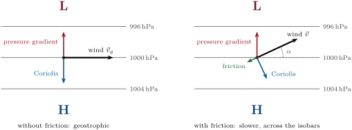
Proposition 28.8 (Friction turns the wind towards low pressure)

Suppose a steady horizontal wind $\vec v$ is acted on by the pressure-gradient force, the Coriolis force and a friction force $-\vec v/\tau$ , with $\tau > 0$ , at a latitude where $f > 0$ . Then the wind crosses the isobars towards low pressure at the angle $\alpha$ with $\tan\alpha = 1/(f\tau)$ , and its speed is $|\vec v| = |\vec v_g|\cos\alpha$ , less than the geostrophic wind.

Proof. Let $V = |\vec v|$ , $\hat v$ the unit vector along the wind and $\hat n$ the unit vector at right angles to it, to its left. The balance is $-(1/\rho)\nabla p - f\, \vec k\times\vec v - \vec v/\tau = \vec 0$ , and $\vec k\times\vec v = V\hat n$ . Along $\hat v$ : $-(1/\rho)\,\nabla p\cdot\hat v = V/\tau > 0$ , so the wind has a component down the pressure gradient, towards low pressure. Along $\hat n$ : $-(1/\rho)\,\nabla p\cdot\hat n = fV$ . The pressure-gradient force, of size $P = |\nabla p|/\rho = f|\vec v_g|$ , therefore has components $V/\tau$ along the wind and $fV$ across it: it makes with the wind the angle $\beta$ with $\tan\beta = 1/(f\tau)$ , and $P^2 = V^2(f^2 + 1/\tau^2)$ . The isobars are perpendicular to the gradient, so the wind crosses them at $\alpha = \beta$ , and $V = P/\sqrt{f^2 + 1/\tau^2} = (P/f)\cos\alpha = |\vec v_g|\cos\alpha$ . ∎

A rougher surface means a stronger drag, a shorter $\tau$ and a larger angle: the wind crosses the isobars more steeply over land than over the sea. Real friction is not exactly linear in the wind, but the conclusion, slower and turned towards the low, is general.

Remark 28.9 (The gradient wind)

Around a centre the isobars are curved, and air that follows them is accelerated towards the centre of curvature, $V^2/r$ for a circle of radius $r$ . Around a low in the Northern Hemisphere, the pressure-gradient force must then exceed the Coriolis force: $fV + V^2/r = f|\vec v_g|$ , and the wind, called the gradient wind, is weaker than the geostrophic one. Around a high, the Coriolis force must exceed the pressure-gradient force, $fV - V^2/r = f|\vec v_g|$ : the wind is stronger, but the equation has a solution only if $|\vec v_g| \leq fr/4$ , which forbids strong pressure gradients near the centre of an anticyclone (Exercise 28.10).

28.3 Depressions and anticyclones

Definition 28.10 (Cyclone, anticyclone)

A cyclone is a large-scale circulation of winds around a centre of low pressure, a depression; an anticyclone is a circulation around a centre of high pressure. A cyclone turns anticlockwise in the Northern Hemisphere and clockwise in the Southern; an anticyclone the other way round.

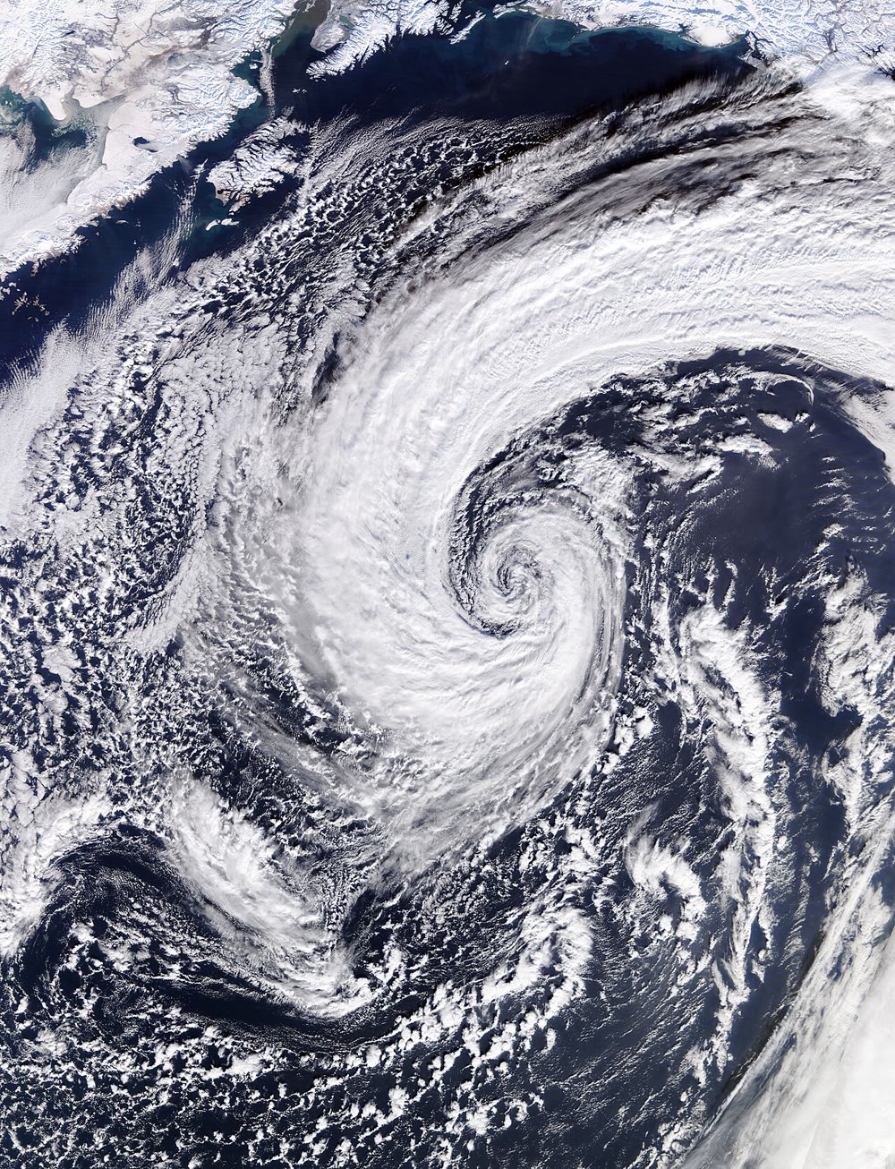
The senses of rotation follow from Theorem 28.6: in the Northern Hemisphere, a wind that keeps the low on its left goes round the low anticlockwise and round a high clockwise. Seen from space, the clouds of a depression trace the turning (the photograph at the head of the chapter); in the Southern Hemisphere the spirals are mirror images.

History — Buys Ballot’s law, 1857

In 1857 the Dutch meteorologist C. H. D. Buys Ballot stated a rule found in the observations: in the Northern Hemisphere, a person standing with their back to the wind has low pressure on the left and high pressure on the right; in the Southern Hemisphere, the reverse. He did not know that the American meteorologist William Ferrel had already deduced it from theory, and later acknowledged Ferrel’s priority. The geostrophic wind is the law in equations.

Friction adds an important twist. Near the ground the wind crosses the isobars towards low pressure (Proposition 28.8): around a depression the air spirals inwards, converges near the ground, and must rise. Rising air expands and cools at the dry adiabatic lapse rate (Chapter 26), and once it is saturated its water vapour condenses: depressions bring cloud and rain. Around an anticyclone the surface air spirals outwards; air sinks from above to replace it, warms by compression, and its clouds evaporate: anticyclones bring settled, often clear weather.

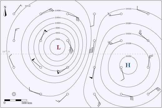
The map below is an invented example, computed rather than observed: a depression $28\,\mathrm{hPa}$ deep and an anticyclone $20\,\mathrm{hPa}$ high on a background of $1013\,\mathrm{hPa}$ , centred near $50{}^{\circ}$ N. At each station the wind barb shows the geostrophic wind computed from the map with Theorem 28.6.

An invented sea-level pressure map near 50 N (isobars every 4\, hPa; central pressures 986\, hPa and 1033\, hPa). Each barb points into the geostrophic wind at its station, the staff towards where the wind comes from; a full feather is 10\, kn, a half feather 5\, kn, a pennant 50\, kn (1\, kn = 0.514\, m/ s). The winds turn anticlockwise round the low and clockwise round the high, and are strongest where the isobars crowd between the two, reaching 36\, m/ s. — An invented sea-level pressure map near $50{}^{\circ}$ N (isobars every $4\,\mathrm{hPa}$ ; central pressures $986\,\mathrm{hPa}$ and $1033\,\mathrm{hPa}$ ). Each barb points into the geostrophic wind at its station, the staff towards where the wind comes from; a full feather is $10\,\mathrm{kn}$ , a half feather $5\,\mathrm{kn}$ , a pennant $50\,\mathrm{kn}$ ( $1\,\mathrm{kn}$ = $0.514\,\mathrm{m}/\mathrm{s}$ ). The winds turn anticlockwise round the low and clockwise round the high, and are strongest where the isobars crowd between the two, reaching $36\,\mathrm{m}/\mathrm{s}$ .

28.4 The three-cell circulation

Averaged round the globe and over many years, the winds that blow north or south are weak, a few metres per second at most, but they carry a lot of air. Their pattern is best seen in the mass that flows between the equator and the poles.

Definition 28.11 (Mean meridional streamfunction)

The mean meridional streamfunction $\psi(p, \varphi)$ is the mass of air per second that crosses the latitude $\varphi$ northwards above the pressure level $p$ , in the zonal and time mean:

\psi(p, \varphi) = \frac{2\pi a_\oplus\cos\varphi}{g}\int_0^p [v]\,\mathrm dp' ,

where $[v]$ is the northward wind averaged round the parallel. It is measured in $\mathrm{kg}\,\mathrm{s}^{-1}$ .

Since $\mathrm dp' = -\rho g\,\mathrm dz$ by the hydrostatic relation, $2\pi a_\oplus \cos\varphi\,[v]\,\mathrm dp'/g$ is the mass flux through a ring of the parallel. The air crossing the parallel above $p$ must cross it the other way below $p$ , since mass does not pile up: $\psi$ vanishes at the ground and at the top, and its lines of equal value are the paths of the mean circulation. A cell with $\psi > 0$ turns clockwise when drawn with the North Pole on the right: northward above, southward below.

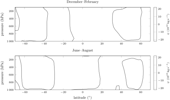
The mean meridional streamfunction in the northern winter (top) and the northern summer (bottom), from the zonal-mean northward wind of the NCEP-NCAR Reanalysis 1, means 1991–2020 (data provided by the NOAA PSL). Red: clockwise cells in this view (rising on their southern side), blue: anticlockwise; black: the zero lines that separate the cells. The winter Hadley cell straddles the equator and dwarfs the summer one.

In the annual mean the reanalysis shows two strong cells astride the equator, with maxima of $8.7 \times 10^{10}\,\mathrm{kg}/\mathrm{s}$ near $15{}^{\circ}$ N and $15{}^{\circ}$ S at $400\,\mathrm{hPa}$ ; at $500\,\mathrm{hPa}$ their poleward edges lie at $33{}^{\circ}$ N and $32{}^{\circ}$ S. Poleward of them, two weaker cells turn the other way, out to about $61{}^{\circ}$ N and $64{}^{\circ}$ S. The seasons reshape the picture: in December to February, the northern winter, the cell that rises south of the equator and sinks in the northern subtropics carries $21.4 \times 10^{10}\,\mathrm{kg}/\mathrm{s}$ and reaches from $13{}^{\circ}$ S to $31{}^{\circ}$ N; in June to August its mirror image carries $18.9 \times 10^{10}\,\mathrm{kg}/\mathrm{s}$ from $17{}^{\circ}$ N to $29{}^{\circ}$ S.

Definition 28.12 (Hadley, Ferrel and polar cells; subtropical high)

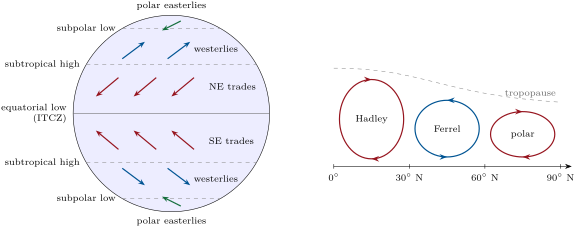
The mean meridional circulation of each hemisphere has three cells. The Hadley cell rises near the equator, flows poleward aloft, sinks near $30{}^{\circ}$ and returns towards the equator at the surface. The Ferrel cell, between about $30{}^{\circ}$ and $60{}^{\circ}$ , turns the opposite way: sinking near $30{}^{\circ}$ and rising near $60{}^{\circ}$ , its surface flow poleward. The polar cell, the smallest and weakest, rises near $60{}^{\circ}$ , sinks over the pole and returns towards $60{}^{\circ}$ at the surface. The subtropical highs are the belts of high sea-level pressure near $30{}^{\circ}$ N and S, under the sinking branches of the Hadley cells.

Definition 28.13 (Trade winds, westerlies)

The trade winds are the persistent surface winds that blow from the subtropical highs towards the equatorial low, turned by the Coriolis force into north-easterlies in the Northern Hemisphere and south-easterlies in the Southern. The westerlies are the prevailing winds from the west of the mid-latitudes, between about $35{}^{\circ}$ and $60{}^{\circ}$ . Poleward of them blow the polar easterlies.

The surface branch of each cell explains its wind. The return flow of the Hadley cell moves towards the equator and is turned to the west by the Coriolis force: the trade winds. The surface flow of the Ferrel cell moves poleward and is turned to the east: the westerlies. In the reanalysis’s annual mean, the zonal wind just above the ground is $-3.5\,\mathrm{m}/\mathrm{s}$ at $15{}^{\circ}$ N and $-4.4\,\mathrm{m}/\mathrm{s}$ at $15{}^{\circ}$ S (negative: from the east), $+1.9\,\mathrm{m}/\mathrm{s}$ at $45{}^{\circ}$ N and $+6.5\,\mathrm{m}/\mathrm{s}$ at $45{}^{\circ}$ S; the sea-level pressure peaks at $1017.5\,\mathrm{hPa}$ near $35{}^{\circ}$ N and $1018.7\,\mathrm{hPa}$ near $32{}^{\circ}$ S, and falls to $988\,\mathrm{hPa}$ at $60{}^{\circ}$ S, the deep trough of the Southern Ocean.

Left: the surface winds of the three-cell circulation, turned to the right of their motion in the Northern Hemisphere and to the left in the Southern, between the pressure belts. Right: the three cells of the Northern Hemisphere on a meridional section (height not to scale); the Southern Hemisphere is the mirror image. The trade winds are the return branch of the Hadley cell, the westerlies the surface branch of the Ferrel cell.

History — Hadley 1735, Ferrel 1856

In 1735 George Hadley published in the Philosophical Transactions a short paper on the cause of the general trade winds. To explain them he proposed a single circulation in each hemisphere, from the equator to the pole. In 1856 William Ferrel published An essay on the winds and currents of the ocean, in which the air of the middle latitudes flows towards the pole and eastward near the surface: the first account of the westerlies between $35{}^{\circ}$ and $60{}^{\circ}$ . His paper gave no mathematical justification; the circulation he described is the cell that bears his name.

Why should the Hadley cell stop near $30{}^{\circ}$ rather than run to the pole, as Hadley thought? The answer lies in the angular momentum the air carries about the Earth’s axis.

Proposition 28.14 (The angular-momentum wind)

A ring of air at latitude $\varphi$ , with eastward wind $u$ relative to the ground, has the absolute angular momentum per unit mass about the Earth’s axis $M = (\Omega a_\oplus\cos\varphi + u)\,a_\oplus\cos\varphi$ . If a ring at rest at the latitude $\varphi_0$ moves to $\varphi$ with no torque acting on it, it arrives with the wind

u(\varphi) = \Omega a_\oplus\,\frac{\cos^2\varphi_0 - \cos^2\varphi}{\cos\varphi}, \qquad\text{and from the equator}\qquad u(\varphi) = \Omega a_\oplus\,\frac{\sin^2\varphi}{\cos\varphi} .

Proof. A ring at latitude $\varphi$ is at the distance $r = a_\oplus\cos\varphi$ from the axis. Its absolute eastward speed is that of the ground, $\Omega r$ , plus the wind $u$ ; its angular momentum per unit mass is $M = (\Omega r + u)\,r$ . Without torque, $M$ is conserved: $(\Omega a_\oplus\cos\varphi + u)\cos\varphi = \Omega a_\oplus \cos^2\varphi_0$ , whence the first formula; $\varphi_0 = 0$ gives the second, since $1 - \cos^2\varphi = \sin^2\varphi$ . ∎

The ground at the equator moves east at $\Omega a_\oplus = 464.6\,\mathrm{m}/\mathrm{s}$ . Air that leaves it at rest aloft and moves poleward comes closer to the axis and, like a skater pulling in her arms, spins faster than the ground beneath it: by $20{}^{\circ}$ it would blow from the west at $58\,\mathrm{m}/\mathrm{s}$ , by $30{}^{\circ}$ at $134\,\mathrm{m}/\mathrm{s}$ , by $40{}^{\circ}$ at $251\,\mathrm{m}/\mathrm{s}$ . No wind of that strength is observed. The zonal-mean wind at $200\,\mathrm{hPa}$ peaks at $42.3\,\mathrm{m}/\mathrm{s}$ near $30{}^{\circ}$ N in the northern winter and $40.4\,\mathrm{m}/\mathrm{s}$ near $30{}^{\circ}$ S in the southern winter.

The eastward wind of a ring of air that leaves the equator at rest and keeps its angular momentum (red, ), against the zonal-mean wind at 200\, hPa in the reanalysis (black: northern winter; dashed: northern summer), NCEP-NCAR Reanalysis 1, means 1991–2020, data provided by the NOAA PSL. The two agree near the equator; poleward of 15 the ring outruns the real wind more and more. — The eastward wind of a ring of air that leaves the equator at rest and keeps its angular momentum (red, Proposition 28.14), against the zonal-mean wind at $200\,\mathrm{hPa}$ in the reanalysis (black: northern winter; dashed: northern summer), NCEP-NCAR Reanalysis 1, means 1991–2020, data provided by the NOAA PSL. The two agree near the equator; poleward of $15{}^{\circ}$ the ring outruns the real wind more and more.

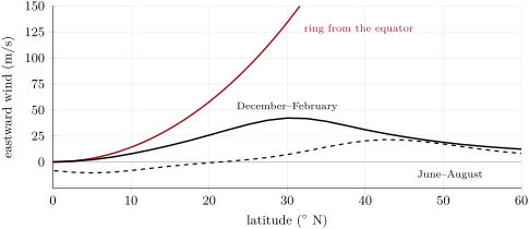
The proposition gives the upper branch of the Hadley cell a limit. As its air moves poleward, its westerly wind grows, and so does the Coriolis force that turns it back towards the equator; long before the ring’s speeds are reached, the flow becomes unstable and breaks into large eddies, the depressions and anticyclones of the mid-latitudes. These eddies, rather than a smooth overturning, carry heat and angular momentum poleward beyond the subtropics; the Ferrel cell is the averaged signature of their motion, and the real jet is slower than the ring because the eddies take part of its angular momentum away. Why the cell ends near $30{}^{\circ}$ rather than at $20{}^{\circ}$ or $40{}^{\circ}$ needs the theory of these instabilities, beyond this volume.

Figures as of 2021

The assessment of the Intergovernmental Panel on Climate Change published in 2021 finds a likely widening of the Hadley circulation since the 1980s, mostly by its extension in the Northern Hemisphere, although with only medium confidence in the extent of the changes, together with a strengthening, particularly in the Northern Hemisphere (medium confidence).

28.5 The ITCZ and the Walker circulation

Definition 28.15 (Intertropical convergence zone)

The intertropical convergence zone (ITCZ) is the belt near the equator where the north-easterly and south-easterly trade winds converge, forming an often continuous band of cloud and thunderstorms. It is the rising branch of the two Hadley cells; the light winds of its surface are the doldrums of the sailors.

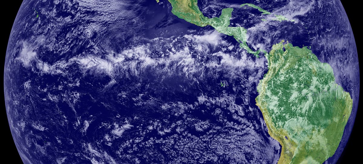
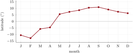
The intertropical convergence zone over the eastern Pacific: a line of bright clouds crossing the ocean north of the equator, with Central and South America to the right. The image combines cloud data from the GOES-11 geostationary satellite with colours of the land cover. (NASA Earth Observatory, public domain, via Wikimedia Commons.)

Converging air must rise, and rising moist air builds clouds: the ITCZ is the rainiest belt of the planet, and its position is traced by the latitude where the zonal-mean precipitation peaks. The ITCZ follows the Sun, with a delay. In the reanalysis the peak moves from $12.8{}^{\circ}$ S in February to $10.9{}^{\circ}$ N in September; averaged over the twelve months it lies at $2.6{}^{\circ}$ N. The zonal mean hides large differences between longitudes: over the eastern Pacific in the photograph the band lies north of the equator, and a zonal mean averages such bands with others that swing farther with the seasons.

The latitude of the zonal-mean precipitation maximum, month by month, between 20 S and 20 N: the intertropical convergence zone migrates north in the northern summer and south in the southern summer, two or three months behind the Sun. NCEP-NCAR Reanalysis 1, means 1991–2020, data provided by the NOAA PSL. — The latitude of the zonal-mean precipitation maximum, month by month, between $20{}^{\circ}$ S and $20{}^{\circ}$ N: the intertropical convergence zone migrates north in the northern summer and south in the southern summer, two or three months behind the Sun. NCEP-NCAR Reanalysis 1, means 1991–2020, data provided by the NOAA PSL.

Along the equator itself, where $f = 0$ , the air moves straight down the pressure gradient, and an east–west circulation appears over the Pacific.

Definition 28.16 (Walker circulation)

The Walker circulation is the east–west overturning cell of the atmosphere along the equatorial Pacific: air rises over the warm waters of the west, around the Maritime Continent, flows east aloft, sinks over the eastern Pacific and returns westward near the surface with the trade winds.

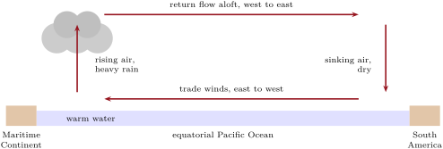
The Walker circulation along the equatorial Pacific (schematic; height not to scale): rising over the warm west, eastward aloft, sinking in the east and back westward with the trade winds near the surface.

The Walker circulation is not steady. When it weakens, the rising motion over the Maritime Continent weakens and the air there may even sink; when it strengthens, the rising and the rain over the west increase. These swings, El Niño and La Niña, and the seasonal reversals of the monsoons are the subject of the Year 2 volume. Over the decades since 1980, the 2021 assessment of the IPCC finds a very likely strengthening of the Walker circulation, resembling the La Niña state, and a westward shift, with medium confidence in the size of the changes.

28.6 Jet streams

Definition 28.17 (Jet stream; subtropical and polar-front jets)

A jet stream is a narrow band of strong wind, normally a horizontal wind high in the troposphere, whose position changes from day to day. The subtropical jet blows from the west near the poleward edge of the Hadley cell, usually between $20{}^{\circ}$ and $30{}^{\circ}$ of latitude at heights of $12\text{ to }14\,\mathrm{km}$ . The polar-front jet blows from the west above the boundary between polar and subtropical air, between about $50{}^{\circ}$ and $60{}^{\circ}$ ; it is the fast core of the westerlies, steered by and steering the depressions and anticyclones of the mid-latitudes.

Jet streams are typically found around $9\,\mathrm{km}$ , can reach more than $440\,\mathrm{km}/\mathrm{h}$ , and are strongest in the winter of each hemisphere, when the contrast of temperature between the tropics and the pole is largest. The subtropical jet is the angular-momentum wind of Proposition 28.14, tamed by the eddies; it sits at the edge of the Hadley cell, near $30{}^{\circ}$ in the winter mean. The polar-front jet wanders north and south with the passing depressions, and averaging round the globe smears it out: in the zonal mean of the northern summer only a weak maximum of $21.6\,\mathrm{m}/\mathrm{s}$ remains near $42.5{}^{\circ}$ N, and in the southern summer $29.9\,\mathrm{m}/\mathrm{s}$ near $47.5{}^{\circ}$ S. Why the wind increases with height wherever the temperature falls towards the pole, the thermal wind, is shown in the Year 3 volume.

28.7 Exercises

Exercise 28.1 ★

Take $\Omega = 7.292 \times 10^{-5}\,\mathrm{rad}\,\mathrm{s}^{-1}$ . (a) Compute the Coriolis parameter at $0{}^{\circ}$ , $30{}^{\circ}$ , $45{}^{\circ}$ and $90{}^{\circ}$ N. (b) Compute the horizontal Coriolis acceleration of a wind of $10\,\mathrm{m}/\mathrm{s}$ at $45{}^{\circ}$ N and compare it with $g = 9.81\,\mathrm{m}\,\mathrm{s}^{-2}$ . (c) In which direction does it point if the wind blows towards the north?

Solution

Solution of Exercise 28.1.

(a) $f = 2\Omega\sin\varphi$ : $0$ at the equator, $7.29 \times 10^{-5}\,\mathrm{s}^{-1}$ at $30{}^{\circ}$ , $1.031 \times 10^{-4}\,\mathrm{s}^{-1}$ at $45{}^{\circ}$ and $1.458 \times 10^{-4}\,\mathrm{s}^{-1}$ at the pole. (b) $fV = 1.031 \times 10^{-4} \times 10 = 1.03 \times 10^{-3}\,\mathrm{m}\,\mathrm{s}^{-2}$ , about $1.05 \times 10^{-4}$ of $g$ . (c) In the Northern Hemisphere the deflection is to the right of the motion: a wind blowing towards the north is pushed towards the east.

Exercise 28.2 ★

Two isobars $4\,\mathrm{hPa}$ apart are $400\,\mathrm{km}$ apart at sea level, where $\rho = 1.225\,\mathrm{kg}\,\mathrm{m}^{-3}$ . (a) Compute the acceleration due to the pressure-gradient force. (b) If nothing else acted, how long would it take to accelerate still air to $10\,\mathrm{m}/\mathrm{s}$ ? (c) Compare this acceleration with the Coriolis acceleration of a wind of $10\,\mathrm{m}/\mathrm{s}$ at $45{}^{\circ}$ N, and say what this suggests.

Solution

Solution of Exercise 28.2.

(a) $|\nabla p|/\rho = (400/4 \times 10^{5})/1.225 = 8.16 \times 10^{-4}\,\mathrm{m}\,\mathrm{s}^{-2}$ . (b) $10/8.16 \times 10^{-4} = 12\,250\,\mathrm{s}$ , $3.4\,\mathrm{h}$ . (c) The Coriolis acceleration of a wind of $10\,\mathrm{m}/\mathrm{s}$ at $45{}^{\circ}$ N is $1.03 \times 10^{-3}\,\mathrm{m}\,\mathrm{s}^{-2}$ : the two are of the same size (ratio $0.79$ ). Within a few hours of starting to move, the air feels a Coriolis force able to balance the pressure gradient: the wind settles near the geostrophic speed, here $8.16 \times 10^{-4}/1.031 \times 10^{-4} = 7.9\,\mathrm{m}/\mathrm{s}$ , instead of accelerating down the gradient.

Exercise 28.3 ★

At $40{}^{\circ}$ N, isobars $4\,\mathrm{hPa}$ apart are $250\,\mathrm{km}$ apart; take $\rho = 1.225\,\mathrm{kg}\,\mathrm{m}^{-3}$ . (a) Compute the geostrophic wind in $\mathrm{m}/\mathrm{s}$ and in knots ( $1\,\mathrm{kn}$ = $0.5144\,\mathrm{m}/\mathrm{s}$ ). (b) The low lies to the south. From which direction does the wind blow? (c) Describe the wind barb (staff and feathers) a forecaster would draw.

Solution

Solution of Exercise 28.3.

(a) $f = 2 \times 7.292 \times 10^{-5} \times \sin40{}^{\circ} = 9.374 \times 10^{-5}\,\mathrm{s}^{-1}$ ; $|\vec v_g| = (400/2.5 \times 10^{5})/(1.225 \times 9.374 \times 10^{-5}) = 13.9\,\mathrm{m}/\mathrm{s}$ , or $13.93/0.5144 = 27.1\,\mathrm{kn}$ . (b) In the Northern Hemisphere the wind keeps the low on its left: with the low to the south, it blows towards the west, from the east (azimuth $90{}^{\circ}$ ). (c) The staff points east from the station circle, into the wind; $27.1\,\mathrm{kn}$ rounds to $25\,\mathrm{kn}$ , two full feathers and a half feather, drawn on the clockwise side of the staff, here its southern side, towards the low.

Exercise 28.4 ★

The reanalysis’s annual means give, near the ground, the eastward wind $-3.5\,\mathrm{m}/\mathrm{s}$ at $15{}^{\circ}$ N, $-4.4\,\mathrm{m}/\mathrm{s}$ at $15{}^{\circ}$ S, $+1.9\,\mathrm{m}/\mathrm{s}$ at $45{}^{\circ}$ N and $+6.5\,\mathrm{m}/\mathrm{s}$ at $45{}^{\circ}$ S, and the sea-level pressure $1011.8\,\mathrm{hPa}$ at $15{}^{\circ}$ N, $1016.8\,\mathrm{hPa}$ at $30{}^{\circ}$ N and $1015.8\,\mathrm{hPa}$ at $45{}^{\circ}$ N. (a) Name the wind belt at each of the four latitudes. (b) Explain the sign of each wind with the surface branch of a cell. (c) Where is the subtropical high of the Northern Hemisphere according to these pressures?

Solution

Solution of Exercise 28.4.

(a) $15{}^{\circ}$ N: north-east trade winds; $15{}^{\circ}$ S: south-east trade winds; $45{}^{\circ}$ N and $45{}^{\circ}$ S: westerlies. (b) At $15{}^{\circ}$ the surface air of the Hadley cell returns towards the equator and is turned to the west by the Coriolis force (right in the north, left in the south): easterly, negative $u$ . At $45{}^{\circ}$ the surface air of the Ferrel cell moves poleward and is turned to the east: westerly, positive $u$ . (c) Of the three latitudes, the pressure is highest at $30{}^{\circ}$ N, $1016.8\,\mathrm{hPa}$ : the subtropical high lies near $30{}^{\circ}$ N (the full profile puts its maximum near $35{}^{\circ}$ N).

Exercise 28.5 ★★

A pressure gradient of $2\,\mathrm{hPa}$ per $500\,\mathrm{km}$ , with $\rho = 1.225\,\mathrm{kg}\,\mathrm{m}^{-3}$ , is found at $60{}^{\circ}$ , $50{}^{\circ}$ , $30{}^{\circ}$ , $20{}^{\circ}$ , $10{}^{\circ}$ and $5{}^{\circ}$ N. (a) Compute the geostrophic wind at each latitude. (b) Real winds of the deep tropics rarely exceed a few metres per second over such gradients. Explain why the geostrophic balance fails near the equator, using the time $1/f$ the Coriolis force needs to turn the wind.

Solution

Solution of Exercise 28.5.

(a) $|\nabla p|/\rho = (200/5 \times 10^{5})/1.225 = 3.27 \times 10^{-4}\,\mathrm{m}\,\mathrm{s}^{-2}$ , divided by $f$ : $2.6\,\mathrm{m}/\mathrm{s}$ at $60{}^{\circ}$ , $2.9\,\mathrm{m}/\mathrm{s}$ at $50{}^{\circ}$ , $4.5\,\mathrm{m}/\mathrm{s}$ at $30{}^{\circ}$ , $6.5\,\mathrm{m}/\mathrm{s}$ at $20{}^{\circ}$ , $12.9\,\mathrm{m}/\mathrm{s}$ at $10{}^{\circ}$ and $25.7\,\mathrm{m}/\mathrm{s}$ at $5{}^{\circ}$ . (b) The Coriolis force turns a wind in a time of order $1/f$ : $2.2\,\mathrm{h}$ at $60{}^{\circ}$ , $11\,\mathrm{h}$ at $10{}^{\circ}$ , $22\,\mathrm{h}$ at $5{}^{\circ}$ , and infinitely long at the equator. Near the equator the pressure field changes, and friction acts, long before the wind can be turned along the isobars: the balance never sets in, and the air flows partly down the gradient, at modest speeds.

Exercise 28.6 ★★

(a) With Proposition 28.14, compute the wind of a ring of air that leaves the equator at rest, at $10{}^{\circ}$ , $15{}^{\circ}$ , $20{}^{\circ}$ and $30{}^{\circ}$ ; take $\Omega a_\oplus = 464.6\,\mathrm{m}/\mathrm{s}$ . (b) The same for a ring that starts at rest at $10{}^{\circ}$ , at $15{}^{\circ}$ , $20{}^{\circ}$ and $30{}^{\circ}$ . (c) The rising branch of the Hadley cell is spread over latitudes rather than placed exactly at the equator. How does this change the predicted jet?

Solution

Solution of Exercise 28.6.

(a) $u = 464.6\,\sin^2\varphi/\cos\varphi$ : $14.2\,\mathrm{m}/\mathrm{s}$ at $10{}^{\circ}$ , $32.2\,\mathrm{m}/\mathrm{s}$ at $15{}^{\circ}$ , $57.8\,\mathrm{m}/\mathrm{s}$ at $20{}^{\circ}$ , $134.1\,\mathrm{m}/\mathrm{s}$ at $30{}^{\circ}$ . (b) $u = 464.6\,(\cos^210{}^{\circ} - \cos^2\varphi)/\cos\varphi$ : $17.7\,\mathrm{m}/\mathrm{s}$ at $15{}^{\circ}$ , $42.9\,\mathrm{m}/\mathrm{s}$ at $20{}^{\circ}$ , $117.9\,\mathrm{m}/\mathrm{s}$ at $30{}^{\circ}$ . (c) Air that starts farther from the equator starts closer to the axis, with less angular momentum to spare: it arrives with a weaker westerly at each latitude. Spreading the rising branch lowers the predicted jet, though not nearly enough to reach the observed $40\,\mathrm{m}/\mathrm{s}$ .

Exercise 28.7 ★★

(a) A ship in the Northern Hemisphere has the wind from the south-west. Using Buys Ballot’s law, where is the centre of low pressure? (b) A ship in the Southern Hemisphere has the wind from the north-west. Where is the low? (c) Near the ground the wind crosses the isobars towards low pressure. Does this change your answer to (a) by turning the direction of the low clockwise or anticlockwise?

Solution

Solution of Exercise 28.7.

(a) The wind blows towards the north-east. With one’s back to it, facing north-east, the low is on the left: to the north-west. (b) The wind blows towards the south-east; in the Southern Hemisphere the low is on the right of a person with their back to the wind: to the south-west. (c) The surface wind is turned from the isobars towards the low, that is anticlockwise from the geostrophic wind in the Northern Hemisphere. The geostrophic wind, and the low at right angles to its left, are therefore turned clockwise from the answer of (a): the low lies between north-west and north, at the azimuth $315{}^{\circ} + \alpha$ for a crossing angle $\alpha$ .

Exercise 28.8 ★★

(a) Compute the mass of air between the equator and $30{}^{\circ}$ N and between the pressure levels $1000\,\mathrm{hPa}$ and $100\,\mathrm{hPa}$ , with $a_\oplus = 6371\,\mathrm{km}$ and $g = 9.81\,\mathrm{m}\,\mathrm{s}^{-2}$ . (b) In the annual mean the reanalysis’s northern Hadley cell carries $8.7 \times 10^{10}\,\mathrm{kg}/\mathrm{s}$ . How long would it take to pass that mass through the cell once? (c) Same question with the northern-winter cell, $21.4 \times 10^{10}\,\mathrm{kg}/\mathrm{s}$ .

Solution

Solution of Exercise 28.8.

(a) The area between the equator and $30{}^{\circ}$ N is $2\pi a_\oplus^2\sin30{}^{\circ} = 1.275 \times 10^{14}\,\mathrm{m}^{2}$ ; the mass above a square metre between the two levels is $\Delta p/g = 9 \times 10^{4}/9.81 = 9174\,\mathrm{kg}$ ; the total is $1.170 \times 10^{18}\,\mathrm{kg}$ . (b) $1.170 \times 10^{18}/8.7 \times 10^{10} = 1.34 \times 10^{7}\,\mathrm{s}$ , about $156$ days, five months. (c) $1.170 \times 10^{18}/21.4 \times 10^{10} = 5.47 \times 10^{6}\,\mathrm{s}$ , about $63$ days, two months.

Exercise 28.9 ★★

Suppose that under a subtropical high the air sinks at $1\,\mathrm{cm}/\mathrm{s}$ , and that it is unsaturated. (a) How far does it sink in a day? (b) By how much does it warm in a day, if nothing else acts, with the dry adiabatic lapse rate of $9.8\,\mathrm{K}/\mathrm{km}$ ? (c) The air does not warm by that much day after day. Which process of Chapter 27 balances the warming? (d) Why are many of the great hot deserts found under these highs?

Solution

Solution of Exercise 28.9.

(a) $0.01 \times 86\,400 = 864\,\mathrm{m}$ a day. (b) $0.864 \times 9.8 = 8.5\,\mathrm{K}$ a day. (c) The air cools by emitting infrared radiation: the atmosphere loses more energy by radiation than it absorbs, and the descent of the air, warming it by compression, makes up the loss. (d) Sinking air warms and dries relative to saturation, its clouds evaporate and rain cannot form: the subtropical highs are belts of clear skies and little rain, where hot deserts form on land.

Exercise 28.10 ★★★

At $50{}^{\circ}$ N, take $f = 1.117 \times 10^{-4}\,\mathrm{s}^{-1}$ and circular isobars of radius $r = 500\,\mathrm{km}$ (Remark 28.9). (a) Around a low where the geostrophic wind would be $15\,\mathrm{m}/\mathrm{s}$ , solve $V^2/r + fV = f|\vec v_g|$ for the gradient wind $V$ . (b) Around a high, show that $V^2/r - fV + f |\vec v_g| = 0$ has a solution only if $|\vec v_g| \leq fr/4$ , and compute that limit. (c) What does (b) imply for the spacing of the isobars near the centre of an anticyclone, compared with a depression?

Solution

Solution of Exercise 28.10.

(a) $V^2 + frV - fr|\vec v_g| = 0$ with $fr = 55.85\,\mathrm{m}/\mathrm{s}$ : $V = \tfrac12\bigl(-55.85 + \sqrt{55.85^2 + 4 \times 55.85 \times 15}\bigr) = 12.3\,\mathrm{m}/\mathrm{s}$ , $82\,\%$ of the geostrophic wind. (b) $V^2 - frV + fr|\vec v_g| = 0$ has real roots only if $(fr)^2 \geq 4fr|\vec v_g|$ , that is $|\vec v_g| \leq fr/4 = 14.0\,\mathrm{m}/\mathrm{s}$ . (c) Near the centre of a high, where $r$ is small, the limit $fr/4$ is small: the pressure gradient must be weak, the isobars far apart and the winds light. A depression has no such limit: its isobars can crowd close to the centre, with strong winds.

Exercise 28.11 ★★★

(a) Show that for small $\varphi$ (in radians) the wind of a ring leaving the equator at rest is $u \approx \Omega a_\oplus\varphi^2$ . (b) Compare the approximation with the exact formula at $10{}^{\circ}$ , with $\Omega a_\oplus = 464.6\,\mathrm{m}/\mathrm{s}$ . (c) The reanalysis’s annual-mean wind at $200\,\mathrm{hPa}$ peaks at $27.0\,\mathrm{m}/\mathrm{s}$ near $35{}^{\circ}$ N. At what latitude would the ring reach this speed? (d) What does the answer say about how far the angular-momentum argument can be trusted?

Solution

Solution of Exercise 28.11.

(a) For small $\varphi$ , $\sin\varphi \approx \varphi$ and $\cos\varphi \approx 1$ , so $u \approx \Omega a_\oplus\varphi^2$ . (b) $10{}^{\circ} = 0.1745\,\mathrm{rad}$ : $464.6 \times 0.1745^2 = 14.15\,\mathrm{m}/\mathrm{s}$ , against $14.23\,\mathrm{m}/\mathrm{s}$ exactly, $0.5\,\%$ less. (c) Solving $464.6\sin^2\varphi/\cos\varphi = 27.0$ numerically gives $\varphi = 13.7{}^{\circ}$ . (d) The ring already matches the real annual-mean jet at less than $14{}^{\circ}$ : conservation of angular momentum describes the upper branch of the Hadley cell only in the deep tropics; poleward of about $15{}^{\circ}$ , the eddies take over.

Exercise 28.12 ★★★

The reanalysis’s zonal-mean precipitation peaks at the following latitudes, from January to December: $-10.5{}^{\circ}$ , $-12.8{}^{\circ}$ , $-5.8{}^{\circ}$ , $-4.6{}^{\circ}$ , $5.5{}^{\circ}$ , $7.3{}^{\circ}$ , $8.6{}^{\circ}$ , $10.4{}^{\circ}$ , $10.9{}^{\circ}$ , $9.1{}^{\circ}$ , $7.4{}^{\circ}$ , $6.2{}^{\circ}$ (negative: south). (a) Compute the annual mean and the range. (b) The subsolar latitude is extreme in June and December. By how many months does the ITCZ lag behind it, and what in the climate system can store heat to cause such a lag? (c) Suppose that over one ocean the ITCZ stays north of the equator all year. Explain how the zonal mean can still cross the equator.

Solution

Solution of Exercise 28.12.

(a) Mean $31.7/12 = 2.6{}^{\circ}$ N; range from $12.8{}^{\circ}$ S to $10.9{}^{\circ}$ N, that is $23.7{}^{\circ}$ . (b) The northernmost position comes in September, three months after the June solstice; the southernmost in February, two months after the December solstice. The lag comes from heat storage, above all in the mixed layer of the ocean (Chapter 26), which warms and cools slowly. (c) The zonal mean averages all longitudes: if over the continents the band of rain swings far into the summer hemisphere, the mean of all longitudes can cross the equator although the band over one ocean does not.

28.8 Problem: Reading a mid-latitude weather map

Problem 28.1

Weekend problem — the wind at a station near $50{}^{\circ}$ N

A weather map of the North Atlantic shows, near a station P at $50{}^{\circ}$ N, straight isobars running west to east, every $4\,\mathrm{hPa}$ , with the lower pressures to the north. P lies between the $1004\,\mathrm{hPa}$ and $1008\,\mathrm{hPa}$ isobars, which are $250\,\mathrm{km}$ apart there; its sea-level pressure is $1006\,\mathrm{hPa}$ and its air temperature $10{}^{\circ}\mathrm{C}$ . The map is invented, but its numbers are typical. Use $\Omega = 2\pi/(23.9345\,\mathrm{h})$ , $a_\oplus = 6371\,\mathrm{km}$ , $R_d = 287.05\,\mathrm{J}\,\mathrm{kg}^{-1}\,\mathrm{K}^{-1}$ for dry air, $1\,\mathrm{kn}$ = $0.514\,444\,\mathrm{m}/\mathrm{s}$ .

Part I — The pressure gradient and the geostrophic wind.

Compute the density of the air at P with the ideal-gas law.
Compute the horizontal pressure gradient at P, in $\mathrm{Pa}\,\mathrm{m}^{-1}$ .
Compute the acceleration due to the pressure-gradient force.
Compute $\Omega$ and the Coriolis parameter at $50{}^{\circ}$ N.
Compute the geostrophic wind speed at P.
Express it in knots and in $\mathrm{km}/\mathrm{h}$ .
Show that the time the pressure-gradient force alone would need to bring still air to the geostrophic speed is $1/f$ , and compute it, together with the time $2\pi/f$ the Coriolis force takes to turn a wind full circle.

Part II — Direction and hemisphere.

In which direction does the pressure-gradient force point at P? In which direction does the geostrophic wind blow, and from which azimuth does it come?
Check your answer with Buys Ballot’s law.
Describe the wind barb drawn at P: the direction of the staff, the number of feathers, and the side on which they stand.
Suppose the same isobars, with the low to the north, were found at $50{}^{\circ}$ S. From which direction would the wind blow?
With the same density and pressure gradient, compute the geostrophic wind at $30{}^{\circ}$ N and $60{}^{\circ}$ N.
Compute it at $5{}^{\circ}$ N. Is the result believable? Explain.

Part III — The wind at the ground. An anemometer at P measures a wind of $9.0\,\mathrm{m}/\mathrm{s}$ crossing the isobars at $25{}^{\circ}$ towards low pressure.

Compute the ratio of the observed wind to the geostrophic wind, and the components of the observed wind along and across the isobars.
From which azimuth does the observed wind blow?
In the linear-drag model of Proposition 28.8, what time constant $\tau$ gives the observed angle, and what speed does the model then predict? Compare with the observation.
Around a depression of radius $500\,\mathrm{km}$ , suppose that the air of the lowest kilometre flows inwards everywhere with the cross-isobar component of question 14 and the density of question 1. Compute the mass of air entering the depression per second.
This air must leave through the top of the layer. Compute the mean upward velocity there, in $\mathrm{m}/\mathrm{s}$ and in metres per day.
At the dry adiabatic lapse rate of $9.8\,\mathrm{K}/\mathrm{km}$ , by how much does the rising air cool in a day? What weather follows, and what would happen under an anticyclone instead?

Part IV — The jet above. The zonal-mean wind at $200\,\mathrm{hPa}$ in the northern winter peaks at $42.3\,\mathrm{m}/\mathrm{s}$ near $30{}^{\circ}$ N (reanalysis means 1991–2020).

Compute the eastward speed of the ground at the equator and at $30{}^{\circ}$ N.
A ring of air leaves the equator at rest aloft and keeps its angular momentum. Compute its wind at $20{}^{\circ}$ N and $30{}^{\circ}$ N.
Same question at $30{}^{\circ}$ N for a ring that starts at rest at $10{}^{\circ}$ N.
By what factor does the ring of question 21 outrun the observed jet at $30{}^{\circ}$ N? Give two reasons why the real jet is slower.
Compute the ratio of the absolute angular momentum per unit mass of the observed jet at $30{}^{\circ}$ N to that of air at rest at the equator. What fraction has been lost on the way?
What is the geostrophic wind speed at P, in metres per second, and how does the wind measured at the ground compare with it?

Solution

Solution of Problem 28.1.

$\rho = p/(R_dT) = 100\,600/(287.05 \times 283.15) = 1.238\,\mathrm{kg}\,\mathrm{m}^{-3}$ .
$|\nabla p| = 400\,\mathrm{Pa}/2.5 \times 10^{5}\,\mathrm{m} = 1.6 \times 10^{-3}\,\mathrm{Pa}\,\mathrm{m}^{-1}$ .
$|\nabla p|/\rho = 1.6 \times 10^{-3}/1.238 = 1.293 \times 10^{-3}\,\mathrm{m}\,\mathrm{s}^{-2}$ .
$\Omega = 2\pi/86\,164.2 = 7.292 \times 10^{-5}\,\mathrm{rad}\,\mathrm{s}^{-1}$ ; $f = 2\Omega\sin50{}^{\circ} = 1.117 \times 10^{-4}\,\mathrm{s}^{-1}$ .
$|\vec v_g| = 1.293 \times 10^{-3}/1.117 \times 10^{-4} = 11.57\,\mathrm{m}/\mathrm{s}$ .
$11.57/0.514444 = 22.5\,\mathrm{kn}$ ; $11.57 \times 3.6 = 41.7\,\mathrm{km}/\mathrm{h}$ .
The time is $|\vec v_g|/(|\nabla p|/\rho)$ and $|\vec v_g| = (|\nabla p|/\rho)/f$ , so it is $1/f = 8951\,\mathrm{s}$ , $2.49\,\mathrm{h}$ ; and $2\pi/f = 15.6\,\mathrm{h}$ . Patterns that last a day or more are therefore close to balance.
The pressure-gradient force points north, towards the low. The geostrophic wind blows along the isobars with the low on its left: towards the east, from the west, azimuth $270{}^{\circ}$ : a westerly.
With one’s back to a westerly, facing east, the left is north, where the low lies: the law is satisfied.
The staff points west from the station circle, towards where the wind comes from; $22.5\,\mathrm{kn}$ rounds to $20\,\mathrm{kn}$ , two full feathers; they stand on the clockwise side of the staff, its northern side, towards the low.
At $50{}^{\circ}$ S, $f < 0$ : the wind keeps the low on its right, so it blows towards the west, from the east.
$f(30{}^{\circ}) = 7.292 \times 10^{-5}\,\mathrm{s}^{-1}$ : $17.7\,\mathrm{m}/\mathrm{s}$ ; $f(60{}^{\circ}) = 1.263 \times 10^{-4}\,\mathrm{s}^{-1}$ : $10.2\,\mathrm{m}/\mathrm{s}$ .
$f(5{}^{\circ}) = 1.271 \times 10^{-5}\,\mathrm{s}^{-1}$ gives $101.7\,\mathrm{m}/\mathrm{s}$ , a wind never observed with such gradients. The turning time $1/f$ is $22\,\mathrm{h}$ : the balance has no time to set in, and the formula does not apply.
$9.0/11.57 = 0.778$ ; along the isobars $9.0\cos25{}^{\circ} = 8.16\,\mathrm{m}/\mathrm{s}$ , across them towards the low $9.0\sin25{}^{\circ} = 3.80\,\mathrm{m}/\mathrm{s}$ .
The geostrophic wind blows towards azimuth $90{}^{\circ}$ ; turned $25{}^{\circ}$ towards the low in the north, the surface wind blows towards $65{}^{\circ}$ , from $245{}^{\circ}$ , the west-south-west.
$\tan\alpha = 1/(f\tau)$ gives $\tau = 1/(1.117 \times 10^{-4}\tan25{}^{\circ}) = 1.92 \times 10^{4}\,\mathrm{s}$ , $5.3\,\mathrm{h}$ ; the model predicts $11.57\cos25{}^{\circ} = 10.5\,\mathrm{m}/\mathrm{s}$ , more than the observed $9.0\,\mathrm{m}/\mathrm{s}$ : real friction is not exactly linear in the wind, and slows it more than the model at this angle.
Through a cylinder of radius $R = 500\,\mathrm{km}$ and height $h = 1\,\mathrm{km}$ : $\dot m = 2\pi R h\rho u_r = 2\pi \times 5 \times 10^{5} \times 1000 \times 1.238 \times 3.80 = 1.48 \times 10^{10}\,\mathrm{kg}/\mathrm{s}$ .
$w = \dot m/(\rho\pi R^2) = 2hu_r/R = 2 \times 1000 \times 3.80/5 \times 10^{5} = 0.0152\,\mathrm{m}/\mathrm{s}$ , about $1310\,\mathrm{m}$ a day.
$1.31 \times 9.8 = 12.9\,\mathrm{K}$ a day: the air soon reaches saturation, and the depression fills with cloud and rain. Under an anticyclone the surface air flows outwards, the air above sinks and warms, and the sky clears.
$\Omega a_\oplus = 7.292 \times 10^{-5} \times 6.371 \times 10^{6} = 464.6\,\mathrm{m}/\mathrm{s}$ at the equator; $464.6\cos30{}^{\circ} = 402.3\,\mathrm{m}/\mathrm{s}$ at $30{}^{\circ}$ N.
$u = 464.6\,\sin^2\varphi/\cos\varphi$ : $57.8\,\mathrm{m}/\mathrm{s}$ at $20{}^{\circ}$ N and $134.1\,\mathrm{m}/\mathrm{s}$ at $30{}^{\circ}$ N.
$u = 464.6\,(\cos^210{}^{\circ} - \cos^230{}^{\circ})/\cos30{}^{\circ} = 117.9\,\mathrm{m}/\mathrm{s}$ .
$134.1/42.3 = 3.17$ . The eddies of the mid-latitudes, depressions and anticyclones, take angular momentum from the upper branch and carry it elsewhere; and the air of the cell rises over a band of latitudes rather than at rest on the equator. The zonal mean also averages a meandering jet over all longitudes.
$M/M_0 = (402.3 + 42.3)\cos30{}^{\circ}/464.6 = 0.829$ : the air has lost $17\,\%$ of the angular momentum it would have kept as a free ring.
The geostrophic wind at P is $11.6\,\mathrm{m}/\mathrm{s}$ , from the west; the wind measured at the ground is $9.0\,\mathrm{m}/\mathrm{s}$ , about four fifths of it, and turned $25{}^{\circ}$ towards the low by friction.

本章定义的术语

在术语表中查看全部 957 个术语