10The Earth’s Heat Budget

Under a mountain in the Japanese Alps, in an old mine cavity, a tank holding a thousand tonnes of liquid scintillator watches for faint flashes of light. Most come from antineutrinos made in the nuclear reactors of the country around it, but some come from below: the uranium and thorium inside the Earth emit antineutrinos as they decay, and these pass through the whole planet as if it were empty. In 2135 days of counting the detector recorded 841 candidate events, of which 106 were attributed to the Earth itself. From that handful of flashes, its team estimated in 2011 that the decay of uranium and thorium heats the Earth with about 20 terawatts. The planet as a whole loses about 47. This chapter accounts for the difference: where the Earth’s heat comes from, how the heat flowing out of it is measured, how temperature rises with depth when the heat is carried by conduction, why the mantle must convect, and why the plates are the cold upper boundary of that convection.

You already know

Heat flows from hot to cold; a rock’s thermal conductivity $k$ measures how easily heat crosses it, its thermal diffusivity $\kappa = k/(\rho c)$ how fast a temperature change spreads (physics, University Year 2). Radioactive nuclei decay with a fixed half-life (physics). The temperature rises with depth along the geotherm, and the mantle convects (Book 2, grades 11 and 12). The lithosphere is the strong outer shell of the Earth (Chapter 9).

10.1 Where the heat comes from

Definition 10.1 (Heat flow)

The heat flow $q$ at a point of the Earth’s surface, or surface heat-flow density, is the power of internal origin that crosses the surface there, per unit area, counted positive outwards. It is measured in $\mathrm{W}\,\mathrm{m}^{-2}$, in practice in $\mathrm{mW}\,\mathrm{m}^{-2}$. Integrated over the whole surface, it gives the Earth’s heat loss $Q = \oint q\,\mathrm dS$.

The heat flow has been measured at tens of thousands of sites. A compilation of $38\,347$ measurements, published in 2010, gives the mean values below, with the oceans and the continents counted separately:

The total, rounded to its uncertainty, is $Q = (47 \pm 2)\,\mathrm{TW}$. Two thirds of it leave through the ocean floor, which is younger and thinner than the continents. It is a small flow: the Sun delivers about $173\,000\,\mathrm{TW}$ to the Earth, and the internal heat amounts to $0.03\,\%$ of the energy budget at the surface. But it is the flow that drives volcanoes, plates and mountain building, and it has two sources.

Definition 10.2 (Radiogenic heat production)

The radiogenic heat production $A$ of a rock is the heat released per unit volume and per unit time by the decay of the radioactive nuclei it contains, in $\mathrm{W}\,\mathrm{m}^{-3}$, in practice in $\text{µ}\mathrm{W}\,\mathrm{m}^{-3}$. A rock of density $\rho$ containing mass fractions $C_i$ of the heat-producing elements, each releasing $H_i$ watts per kilogram of element, has

$$A = \rho \sum_i C_i H_i .$$

Four isotopes produce almost all of this heat, because they are long-lived, abundant enough and energetic: $\ce{^{238}U}$, $\ce{^{235}U}$, $\ce{^{232}Th}$ and $\ce{^{40}K}$. The heat per kilogram of each element is the heat per kilogram of its radioactive isotope times that isotope’s share of the element (Exercise 10.3):

Potassium releases thirty thousand times less heat per kilogram than uranium, but it is a major element of many rocks, counted in per cent where uranium and thorium are counted in parts per million. The rocks rich in all three are the granites and their relatives; the poorest are the mantle peridotites. A compilation of $2188$ analyses gives these medians, in $\text{µ}\mathrm{W}\,\mathrm{m}^{-3}$:

The spread within each group is wide: a quarter of granites produce less than $1.74\,\text{µ}\mathrm{W}\,\mathrm{m}^{-3}$, a quarter more than $3.23\,\text{µ}\mathrm{W}\,\mathrm{m}^{-3}$. The continental crust is enriched in these elements, the oceanic crust and the mantle depleted; but the mantle is so large that it still holds a large share of the planet’s heat sources.

Definition 10.3 (Secular cooling)

Secular cooling is the part of the Earth’s heat loss supplied by the slow decrease of the temperature of its interior, mantle and core: the release of heat stored since the planet’s formation, at a rate $-\sum_j M_j c_j\,\mathrm dT_j/\mathrm dt$ for reservoirs of mass $M_j$, specific heat $c_j$ and mean temperature $T_j$.

Energy conservation gives the budget of the whole Earth: the heat lost at the surface is the radiogenic production plus the secular cooling,

The geoneutrinos measure part of the first term: the 2011 result, which combined two detectors, attributes $20\,\mathrm{TW}$ to uranium and thorium, and $\ce{^{40}K}$, whose antineutrinos are too weak to be detected that way, is known to add about $4\,\mathrm{TW}$.

About half of the heat loss is therefore radiogenic, and the other half, about $23\,\mathrm{TW}$, is secular cooling. Part of that cooling is the core’s: the heat crossing the core–mantle boundary is estimated at $5\text{ to }15\,\mathrm{TW}$. These figures are uncertain: the measurement itself carries an uncertainty of about $9\,\mathrm{TW}$, and the geoneutrino results so far only confine the radiogenic part to $15\text{ to }41\,\mathrm{TW}$, while Earth models of different kinds spread from $14\text{ to }46\,\mathrm{TW}$. The total, measured at the surface, is the best-known term of the budget (figure below).

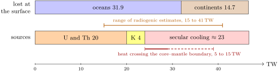
Radiogenic heat was larger in the past, because the isotopes were more abundant: $\ce{^{235}U}$ and $\ce{^{40}K}$, the short-lived ones, then contributed much more (Book 2, grade 12). The Earth’s heat engine is running down slowly, on both counts.

10.2 Measuring the heat flow

Heat flow is not measured directly: it is computed from a temperature gradient and a conductivity.

Proposition 10.4 (Fourier’s law)

In a medium of thermal conductivity $k$, heat is conducted down the temperature gradient at a rate per unit area proportional to it. With $z$ the depth, counted positive downwards, and $q$ counted positive upwards,

$$q = k\,\frac{\mathrm dT}{\mathrm dz} .$$

The law is established in the physics books’ University Year 2 volume. Most rocks conduct heat at $1.5\text{ to }3\,\mathrm{W}\,\mathrm{m}^{-1}\,\mathrm{K}^{-1}$ below $200\,{}^{\circ}\mathrm{C}$, less when hot; models of continental heat flow give the granitic upper crust about $2.7\,\mathrm{W}\,\mathrm{m}^{-1}\,\mathrm{K}^{-1}$;

a gradient of $25\,\mathrm{K}\,\mathrm{km}^{-1}$ in it means a heat flow of about $70\,\mathrm{mW}\,\mathrm{m}^{-2}$.

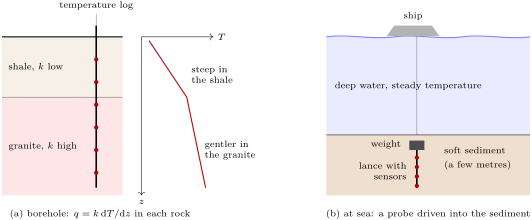
When the rocks crossed by a borehole have different conductivities, the gradient changes from one to the next, but the heat flow does not, as long as no heat is produced or stored between them. The following proposition turns that into a test.

Proposition 10.5 (Bullard plot)

Let $R(z) = \int_0^z \mathrm d\zeta/k(\zeta)$ be the thermal resistance, per unit area, of the rocks between the surface and the depth $z$, in $\mathrm{m}^{2}\,\mathrm{K}\,\mathrm{W}^{-1}$. If the heat flow $q$ is the same at every depth of a borehole, the temperature is a linear function of the thermal resistance: $T(z) = T_0 + q\,R(z)$.

Method 10.6 (The heat flow from a borehole)

1. Log the temperature down the borehole long after drilling, when the disturbance of the drilling fluid has died away, and set aside the shallowest tens of metres, which follow the seasons.
2. Measure the conductivity of core samples of each rock crossed, in the laboratory, and compute the thermal resistance $R(z)$ at each logged depth.
3. Plot $T$ against $R$: the slope of the straight line is the heat flow. A bend reveals water flowing through the rocks, a past change of surface temperature, or an error in a conductivity.
4. Correct, where needed, for the relief, which bends the isotherms below hills and valleys, and for the slow warming since the last glaciation, which still disturbs the upper kilometre or so.

At sea, a borehole is not needed. The temperature at the bottom of the deep ocean is very steady, so that a few metres of soft sediment already carry the equilibrium gradient. A steel lance carrying a row of temperature sensors is dropped from a ship and driven into the sediment by a heavy weight (figure below); the sensors record the gradient, and a heat pulse sent along the lance gives the sediment’s conductivity in place. The ocean floor has one trap. On young crust, sea water circulates through the cracked basalt and carries much of the heat away by advection, so that the measured conductive heat flow falls well short of the true loss. The loss through the youngest ocean floor is therefore computed from the cooling model of Section 10.5, calibrated on old crust where circulation has stopped: this computed part, $23.1\,\mathrm{TW}$, is about half the global total.

In the field — Heat flow at sea

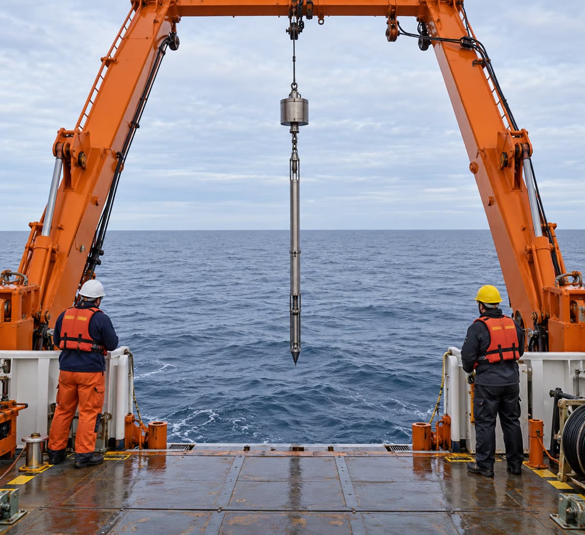
On a research ship, the heat-flow probe is a heavy lance hung from the stern crane. It is lowered on the ship’s cable to just above the sea floor, then let go: the weight drives it into the sediment, and the crew waits on deck while the sensors settle to the temperature of the mud, then pulls it out and moves on to the next station a short way off. A line of such stations across a ridge flank gives the decline of heat flow with the age of the floor, and the scatter between neighbouring stations shows where water is flowing through the crust below.

10.3 The steady conductive geotherm

Definition 10.7 (Geotherm)

The geotherm beneath a point of the surface is the temperature as a function of depth there, $T(z)$. It is a steady conductive geotherm when it does not change with time and heat is carried along it by conduction alone.

Within the lithosphere, far from active volcanoes and from water circulation, the heat is carried by conduction, and on a scale of millions of years the geotherm is steady. Its shape then follows from an energy balance.

Theorem 10.8 (Steady conduction with heat production)

Along a steady conductive geotherm, in a medium of uniform conductivity $k$ with heat production $A(z)$ and no horizontal flow of heat,

$$\frac{\mathrm dq}{\mathrm dz} = -A(z), \qquad\text{that is}\qquad k\,\frac{\mathrm d^2T}{\mathrm dz^2} = -A(z).$$

Read from the surface down, the heat flow decreases with depth by the heat produced above each level: what crosses the surface is the heat coming from below plus all the heat produced on the way. Two distributions of $A$ give closed forms.

Proposition 10.9 (A uniform radiogenic layer)

Let the heat production be $A$ from the surface down to the depth $h$ and zero below, the surface be at temperature $T_0$, and the surface heat flow be $q_0$. Then for $0 \le z \le h$

$$q(z) = q_0 - A z, \qquad T(z) = T_0 + \frac{q_0 z}{k} - \frac{A z^2}{2k},$$

and below $h$ the heat flow is uniform, $q_m = q_0 - A h$, and the geotherm a straight line of slope $q_m/k$.

Theorem 10.10 (Exponential heat production and the linear heat-flow relation)

Let the heat production decrease with depth as $A(z) = A_0 e^{-z/D}$, the heat flow tend to $q_m$ at great depth, and the surface be at $T_0$. Then

$$q(z) = q_m + A_0 D\,e^{-z/D}, \qquad T(z) = T_0 + \frac{q_m z}{k} + \frac{A_0 D^2}{k}\bigl(1 - e^{-z/D}\bigr),$$

and the surface heat flow is

$$q_0 = q_m + A_0 D .$$

The last line is a prediction that can be tested at the surface. Granite plutons in one region share the same deep heat flow $q_m$ and, if they differ only by how rich they are in uranium, thorium and potassium, the same scale $D$; then the heat flow measured over each pluton should be a linear function of the heat production measured on its rocks, with slope $D$, a length, and intercept $q_m$, the reduced heat flow, coming from below the radiogenic layer. Francis Birch first observed such a line, reported in 1968, and the same year three provinces were defined by their lines:

The intercepts, published as 0.8, 1.4 and $0.4\times10^{-6}\,\mathrm{cal}\,\mathrm{cm}^{-2}\,\mathrm{s}^{-1}$, are converted with $1\,\text{µ}\mathrm{cal}\,\mathrm{cm}^{-2}\,\mathrm{s}^{-1} = 41.84\,\mathrm{mW}\,\mathrm{m}^{-2}$ (Exercise 10.4). The slopes vary little, from 7 to $10\,\mathrm{km}$; the reduced heat flow varies a lot, and maps of it show where the mantle below is hot, as under the stretched crust of the Basin and Range. The uniform layer of Proposition 10.9 also gives a straight line, of slope $h$: both models fit the data, but only the exponential one stays a straight line of the same slope when the plutons are eroded to different depths (Exercise 10.10), which is why it is preferred.

Method 10.11 (The temperature at depth beneath a pluton)

1. Measure the surface heat flow $q_0$ over the pluton (borehole method) and its heat production $A_0$ from its U, Th and K contents.
2. From the line of the province, or with a value of $D$ of about $10\,\mathrm{km}$, compute $q_m = q_0 - A_0 D$.
3. Apply Theorem 10.10. Below a few times $D$, $e^{-z/D}$ is negligible and the geotherm is the straight line $T_0 + A_0D^2/k + q_m z/k$: the radiogenic layer has raised every deep temperature by $A_0D^2/k$.

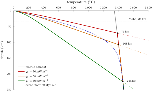
In the figure, the temperature at the Moho ranges from about $320{}^{\circ}\mathrm{C}$ for the lowest heat flow to more than $700{}^{\circ}\mathrm{C}$ for the highest: the heat flow at the surface carries a direct reading of the temperature of the deep crust, which governs its strength (Chapter 16).

10.4 Conduction against convection

Conduction is slow. How slow follows from the heat equation, which the physics books derive from Fourier’s law and the balance of Theorem 10.8 with storage added: in one dimension, without heat production, $\partial T/\partial t = \kappa\,\partial^2 T/\partial z^2$.

Proposition 10.12 (The conductive time scale)

A temperature change imposed at a boundary of a conducting body spreads over a distance $L$ in a time of order

$$\tau = \frac{L^2}{\kappa} .$$

Rocks have $\kappa \approx 10^{-6}\,\mathrm{m}^{2}\,\mathrm{s}^{-1}$. The daily temperature cycle reaches a few tens of centimetres into the ground, the yearly one a few metres, and the warming since the last glaciation a kilometre or so. Across a lithosphere $100\,\mathrm{km}$ thick, $\tau = 10^{16}\,\mathrm{s}$, about $300\,\mathrm{Myr}$. Across the mantle, $2900\,\mathrm{km}$ thick, $\tau = 8.4 \times 10^{18}\,\mathrm{s}$, or $270\,\mathrm{Gyr}$: sixty times the age of the Earth, $4.54\,\mathrm{Gyr}$. Conduction alone could not have brought the heat of the deep mantle anywhere near the surface. The mantle convects, and in its interior the heat is carried by the motion of the rock itself, at the speeds of the plates, centimetres per year.

Definition 10.13 (Mantle adiabat)

The mantle adiabat is the geotherm of the well-mixed interior of the convecting mantle: the temperature that mantle rock takes as it rises or sinks fast enough to exchange no heat with its surroundings, cooling by expansion as it rises and warming by compression as it sinks.

Thermodynamics gives its gradient, $\mathrm dT/\mathrm dz = \alpha g T/c_p$, with $\alpha$ the thermal expansivity and $c_p$ the specific heat (physics, admitted here). It is small. A recent evaluation from mineral physics gives $0.54\,\mathrm{K}\,\mathrm{km}^{-1}$ at $50\,\mathrm{km}$ depth, decreasing to $0.36\,\mathrm{K}\,\mathrm{km}^{-1}$ at $410\,\mathrm{km}$, then 0.41 to $0.23\,\mathrm{K}\,\mathrm{km}^{-1}$ through the lower mantle, with $1646\,\mathrm{K}$ at $50\,\mathrm{km}$ and $2587\,\mathrm{K}$ at $2800\,\mathrm{km}$.

Extrapolated to the surface, the adiabat gives the mantle’s potential temperature, $1619\,\mathrm{K}$ or about $1350{}^{\circ}\mathrm{C}$: the temperature the mantle would have if it were brought up to the surface without exchanging heat. The notion of potential temperature is defined, for the atmosphere and the ocean, in Chapter 26. A temperature that increases by only $0.5\,\mathrm{K}$ per kilometre while the conductive geotherm near the surface climbs by $25\,\mathrm{K}$ is the signature of convection.

History — John Perry and the cooling Earth

In 1862–1863 William Thomson, later Lord Kelvin, computed the age of the Earth from its cooling. He treated it as a solid that had cooled by conduction from a uniform temperature of about $3900{}^{\circ}\mathrm{C}$; with the then mean gradient he chose from the measurements of his time, about $36\,\mathrm{K}\,\mathrm{km}^{-1}$, and a diffusivity of $1.2 \times 10^{-6}\,\mathrm{m}^{2}\,\mathrm{s}^{-1}$, the time needed to reach today’s gradient was about $96\,\mathrm{Myr}$, between bounds of 24 and $400\,\mathrm{Myr}$ (Exercise 10.9). Geologists found this far too short. In 1895, a year before radioactivity was discovered, his former assistant John Perry pointed at an assumption instead: if the interior were partly fluid and convected, it would carry heat as if it had an enormous conductivity, and the whole interior, not a thin outer shell, would feed the surface heat flow. His argument was neglected and forgotten; mantle convection, established long after, proved him right: the deep mantle cools by convection, and that is the secular cooling of the budget.

Proposition 10.14 (Perry’s well-stirred Earth)

Let a sphere of radius $R$ have a well-stirred interior at the uniform temperature $T_i(t)$, with heat capacity $\rho c$ per unit volume, under a conducting lid of thickness $L \ll R$ and conductivity $k$ whose surface is at $0{}^{\circ}\mathrm{C}$, and let there be no heat production. Then

$$T_i(t) = T_i(0)\,e^{-t/\tau_P}, \qquad \tau_P = \frac{RL}{3\kappa},$$

and the surface heat flow $kT_i/L$ decays with the same time constant.

For $R = 6400\,\mathrm{km}$, $L = 100\,\mathrm{km}$ and $\kappa = 10^{-6}\,\mathrm{m}^{2}\,\mathrm{s}^{-1}$, $\tau_P = 6.8\,\mathrm{Gyr}$: a convecting Earth keeps a high heat flow for billions of years, where Kelvin’s conducting Earth lost it in tens of millions (Exercise 10.11).

10.5 The lithosphere as a thermal boundary layer

Definition 10.15 (Thermal boundary layer, thermal lithosphere)

In a convecting fluid, a thermal boundary layer is a layer along a boundary across which heat passes by conduction and the temperature changes from that of the boundary to that of the well-mixed interior. The thermal lithosphere is the upper thermal boundary layer of the mantle: the outer shell of the Earth from the surface down to the depth where the conductive geotherm meets the mantle adiabat.

The plates are the cold top of the mantle’s convection, its upper boundary layer. Their base, where the steep conductive geotherm bends into the gentle adiabat, lies at $70\text{ to }230\,\mathrm{km}$ in the figure of the geotherms for continental heat flows of 70 to $40\,\mathrm{mW}\,\mathrm{m}^{-2}$, in the range measured by seismology (Chapter 9): the lithosphere defined by its strength and the lithosphere defined by its temperature are roughly the same shell, because strength depends on temperature. At the bottom of the mantle, the D$''$ layer is the lower boundary layer, heated from below by the core.

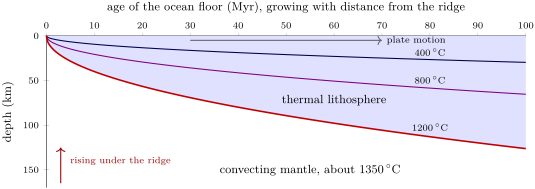
Under the oceans, the boundary layer is born at the ridge, where hot mantle rises to the surface, and thickens as the plate moves away and cools. The cooling of a half-space from a uniform temperature, solved by Fourier and used by Kelvin for the whole Earth, describes it well (Chapter 13 and the Year 3 volume derive it): isotherms deepen as the square root of the age of the floor (figure below), and the heat flow decreases as

the value used in the global budget. At $100\,\mathrm{Myr}$ the half-space has cooled to about $130\,\mathrm{km}$ (Exercise 10.12). The real plate stops thickening sooner: seismic waves crossing the Pacific are best fitted by a cooling plate that tends to a thickness of $85\text{ to }95\,\mathrm{km}$, the flattening of old sea floor met again in Chapter 13.

The heat budget, the heat flow and the thermal structure of the plates come together in the next chapters: the cooling plate subsides (Chapter 13), and the cold lithosphere sinking at subduction zones is the downwelling of the convection it belongs to.

10.6 Exercises

Exercise 10.1 ★

A borehole in granite of conductivity $2.5\,\mathrm{W}\,\mathrm{m}^{-1}\,\mathrm{K}^{-1}$ shows a steady gradient of $22\,\mathrm{K}\,\mathrm{km}^{-1}$. Compute the heat flow, and the power that crosses one square kilometre of the surface there.

Solution

Solution of Exercise 10.1.

$q = k\,\mathrm dT/\mathrm dz = 2.5\times0.022\,\mathrm{K}\,\mathrm{m}^{-1} = 0.055\,\mathrm{W}\,\mathrm{m}^{-2} = 55\,\mathrm{mW}\,\mathrm{m}^{-2}$. Through $1\,\mathrm{km}^{2}$ $= 10^{6}\,\mathrm{m}^{2}$: $5.5 \times 10^{4}\,\mathrm{W}$, that is $55\,\mathrm{kW}$.

Exercise 10.2 ★

From the areas and mean heat flows of the continents ($2.073 \times 10^{14}\,\mathrm{m}^{2}$, $70.9\,\mathrm{mW}\,\mathrm{m}^{-2}$) and the oceans ($3.028 \times 10^{14}\,\mathrm{m}^{2}$, $105.4\,\mathrm{mW}\,\mathrm{m}^{-2}$), compute the heat loss of each, the total and the mean heat flow over the Earth’s surface ($5.101 \times 10^{14}\,\mathrm{m}^{2}$). What fraction of the $173\,000\,\mathrm{TW}$ received from the Sun is it?

Solution

Solution of Exercise 10.2.

Continents $2.073 \times 10^{14}\times0.0709 = 1.470 \times 10^{13}\,\mathrm{W} = 14.70\,\mathrm{TW}$; oceans $3.028 \times 10^{14}\times0.1054 = 31.92\,\mathrm{TW}$; total $46.61\,\mathrm{TW}$, and the mean heat flow $4.661 \times 10^{13}/5.101 \times 10^{14} = 91.4\,\mathrm{mW}\,\mathrm{m}^{-2}$ (the published 46.7 and 91.6 differ only by the rounding of the two means). The fraction of the solar input is $46.6/173000 = 2.7 \times 10^{-4}$, or $0.027\,\%$.

Exercise 10.3 ★

From the table of the four isotopes, compute the heat released per kilogram of natural uranium ($99.274\,\%$ $\ce{^{238}U}$ and $0.720\,\%$ $\ce{^{235}U}$ of the atoms; their masses differ by about $1\,\%$, so take these as mass fractions) and per kilogram of natural potassium, whose $\ce{^{40}K}$ makes $0.0117\,\%$ of the atoms (take the mass of a $\ce{^{40}K}$ atom $39.96/39.10$ times the mean mass of a potassium atom).

Solution

Solution of Exercise 10.3.

Uranium: $0.99274\times9.513 \times 10^{-5} + 0.00720\times5.685 \times 10^{-4} = 9.444 \times 10^{-5} + 4.09 \times 10^{-6} = 9.85 \times 10^{-5}\,\mathrm{W}\,\mathrm{kg}^{-1}$; the rare $\ce{^{235}U}$ supplies $4\,\%$ of it. Potassium: the mass fraction of $\ce{^{40}K}$ is $1.17 \times 10^{-4}\times39.96/39.10 = 1.196 \times 10^{-4}$, so $1.196 \times 10^{-4}\times2.847 \times 10^{-5} = 3.40 \times 10^{-9}\,\mathrm{W}\,\mathrm{kg}^{-1}$.

Exercise 10.4 ★

Convert the intercepts of the three provinces, 0.8, 1.4 and $0.4\times10^{-6}\,\mathrm{cal}\,\mathrm{cm}^{-2}\,\mathrm{s}^{-1}$, into $\mathrm{mW}\,\mathrm{m}^{-2}$ ($1\,\mathrm{cal} = 4.184\,\mathrm{J}$). Predict the surface heat flow over a granite of heat production $3.0\,\text{µ}\mathrm{W}\,\mathrm{m}^{-3}$ in each province.

Solution

Solution of Exercise 10.4.

$1\,\text{µ}\mathrm{cal}\,\mathrm{cm}^{-2}\,\mathrm{s}^{-1} = 4.184 \times 10^{-6}\,\mathrm{J}\,\mathrm{s}^{-1}/10^{-4}\,\mathrm{m}^{2} = 41.84\,\mathrm{mW}\,\mathrm{m}^{-2}$: eastern United States $33.5\,\mathrm{mW}\,\mathrm{m}^{-2}$, Basin and Range $58.6\,\mathrm{mW}\,\mathrm{m}^{-2}$, Sierra Nevada $16.7\,\mathrm{mW}\,\mathrm{m}^{-2}$. With $A_0D$ in $\mathrm{mW}\,\mathrm{m}^{-2}$ when $A_0$ is in $\text{µ}\mathrm{W}\,\mathrm{m}^{-3}$ and $D$ in $\mathrm{km}$: $33.5 + 3.0\times7.5 = 56.0\,\mathrm{mW}\,\mathrm{m}^{-2}$, $58.6 + 3.0\times9.4 = 86.8\,\mathrm{mW}\,\mathrm{m}^{-2}$, $16.7 + 3.0\times10 = 46.7\,\mathrm{mW}\,\mathrm{m}^{-2}$. The same granite gives heat flows almost twice as high in the Basin and Range as in the Sierra Nevada: the difference is in the mantle below.

Exercise 10.5 ★★

A crust has a uniform heat production of $2.0\,\text{µ}\mathrm{W}\,\mathrm{m}^{-3}$ in its upper $10\,\mathrm{km}$ and none below, a conductivity of $2.5\,\mathrm{W}\,\mathrm{m}^{-1}\,\mathrm{K}^{-1}$, a surface heat flow of $60\,\mathrm{mW}\,\mathrm{m}^{-2}$ and a surface temperature of $10{}^{\circ}\mathrm{C}$. Compute the temperature at $10\,\mathrm{km}$, the heat flow below the radiogenic layer, and the temperature at the Moho, $35\,\mathrm{km}$ down.

Solution

Solution of Exercise 10.5.

$T(10\,\text{km}) = 10 + \frac{0.060\times10^4}{2.5} - \frac{2 \times 10^{-6}\times10^8}{2\times2.5} = 10 + 240 - 40 = 210{}^{\circ}\mathrm{C}$. Below, $q_m = 60 - 2.0\times10 = 40\,\mathrm{mW}\,\mathrm{m}^{-2}$, a gradient of $16\,\mathrm{K}\,\mathrm{km}^{-1}$, and $T(35\,\text{km}) = 210 + 16\times25 = 610{}^{\circ}\mathrm{C}$.

Exercise 10.6 ★★

A borehole crosses $300\,\mathrm{m}$ of shale ($k = 1.5\,\mathrm{W}\,\mathrm{m}^{-1}\,\mathrm{K}^{-1}$), then granite ($k = 3.0\,\mathrm{W}\,\mathrm{m}^{-1}\,\mathrm{K}^{-1}$). The equilibrium temperatures are $12.0{}^{\circ}\mathrm{C}$ at the surface, $24.0{}^{\circ}\mathrm{C}$ at $300\,\mathrm{m}$ and $34.0{}^{\circ}\mathrm{C}$ at $800\,\mathrm{m}$. Compute the gradient and the heat flow in each rock, the thermal resistance at $300\,\mathrm{m}$ and at $800\,\mathrm{m}$, and the slope of the Bullard plot. Is the heat flow constant?

Solution

Solution of Exercise 10.6.

Shale: gradient $12.0/0.300 = 40\,\mathrm{K}\,\mathrm{km}^{-1}$, $q = 1.5\times0.040 = 60\,\mathrm{mW}\,\mathrm{m}^{-2}$. Granite: $10.0/0.500 = 20\,\mathrm{K}\,\mathrm{km}^{-1}$, $q = 3.0\times0.020 = 60\,\mathrm{mW}\,\mathrm{m}^{-2}$. $R(300) = 300/1.5 = 200\,\mathrm{m}^{2}\,\mathrm{K}\,\mathrm{W}^{-1}$, $R(800) = 200 + 500/3.0 = 366.7\,\mathrm{m}^{2}\,\mathrm{K}\,\mathrm{W}^{-1}$. The three points $(0, 12.0)$, $(200, 24.0)$, $(366.7, 34.0)$ are aligned, with slope $22.0/366.7 = 0.0600\,\mathrm{W}\,\mathrm{m}^{-2}$: the heat flow is the same, $60\,\mathrm{mW}\,\mathrm{m}^{-2}$, in both rocks; only the gradient changes, in inverse proportion to the conductivity.

Exercise 10.7 ★★

With $\kappa = 10^{-6}\,\mathrm{m}^{2}\,\mathrm{s}^{-1}$, compute the conductive time scale for $L = 1\,\mathrm{m}$, $10\,\mathrm{m}$, $100\,\mathrm{km}$ and $2900\,\mathrm{km}$, each in a suitable unit. Which surface temperature cycles are still felt $10\,\mathrm{m}$ below the ground? Compare the last time with the age of the Earth.

Solution

Solution of Exercise 10.7.

$\tau = L^2/\kappa$: $1\,\mathrm{m}$, $10^{6}\,\mathrm{s}$ or $12$ days; $10\,\mathrm{m}$, $10^{8}\,\mathrm{s}$ or $3.2$ years; $100\,\mathrm{km}$, $10^{16}\,\mathrm{s}$ or $317\,\mathrm{Myr}$; $2900\,\mathrm{km}$, $8.4 \times 10^{18}\,\mathrm{s}$ or $267\,\mathrm{Gyr}$. At $10\,\mathrm{m}$ the daily cycle is not felt at all, and the yearly cycle, shorter than the three years needed to cross $10\,\mathrm{m}$, only very weakly: only changes lasting years or more come through. The last time is $267/4.54 = 59$ times the age of the Earth.

Exercise 10.8 ★★

The mantle adiabat is at $1646\,\mathrm{K}$ at $50\,\mathrm{km}$ depth, with a gradient of $0.54\,\mathrm{K}\,\mathrm{km}^{-1}$ there, decreasing to $0.36\,\mathrm{K}\,\mathrm{km}^{-1}$ at $410\,\mathrm{km}$. (a) Extrapolate it to the surface with the gradient at $50\,\mathrm{km}$, and give the potential temperature in kelvins and in degrees Celsius. (b) Estimate the temperature at $410\,\mathrm{km}$ with the mean of the two gradients, and compare with the published $1799\,\mathrm{K}$ just above the discontinuity.

Solution

Solution of Exercise 10.8.

(a) $1646 - 0.54\times50 = 1619\,\mathrm{K}$, that is $1346{}^{\circ}\mathrm{C}$, the published $1350{}^{\circ}\mathrm{C}$ rounded. (b) Mean gradient $(0.54 + 0.36)/2 = 0.45\,\mathrm{K}\,\mathrm{km}^{-1}$, so $1646 + 0.45\times360 = 1808\,\mathrm{K}$, $9\,\mathrm{K}$ ($0.5\,\%$) above $1799\,\mathrm{K}$: the gradient does not decrease linearly, but the estimate is close.

Exercise 10.9 ★★

A half-space cooled from the uniform temperature $T_0$, its surface held at $0{}^{\circ}\mathrm{C}$, has after a time $t$ the surface gradient $G = T_0/\sqrt{\pi\kappa t}$ (admitted). (a) Express $t$ in terms of $G$. (b) With Kelvin’s values, $T_0 = 3900{}^{\circ}\mathrm{C}$, $\kappa = 1.2 \times 10^{-6}\,\mathrm{m}^{2}\,\mathrm{s}^{-1}$ and $G = 1/50$ of a degree Fahrenheit per foot, compute $G$ in $\mathrm{K}\,\mathrm{km}^{-1}$ and the age. (c) Redo it with $T_0 = 1300{}^{\circ}\mathrm{C}$, $\kappa = 10^{-6}\,\mathrm{m}^{2}\,\mathrm{s}^{-1}$ and $G = 36\,\mathrm{K}\,\mathrm{km}^{-1}$.

Solution

Solution of Exercise 10.9.

(a) $G^2 = T_0^2/(\pi\kappa t)$ gives $t = T_0^2/(\pi\kappa G^2)$. (b) $G = 0.02\times\tfrac59\,\mathrm{K}/0.3048\,\mathrm{m} = 0.036\,45\,\mathrm{K}\,\mathrm{m}^{-1} = 36.45\,\mathrm{K}\,\mathrm{km}^{-1}$; $t = 3900^2/(\pi\times1.2 \times 10^{-6}\times0.03645^2) = 1.521 \times 10^{7}/5.009 \times 10^{-9} = 3.04 \times 10^{15}\,\mathrm{s}$, that is $96\,\mathrm{Myr}$, Kelvin’s figure. (c) $t = 1300^2/(\pi\times10^{-6}\times0.036^2) = 4.15 \times 10^{14}\,\mathrm{s} = 13\,\mathrm{Myr}$: a more realistic initial temperature makes the conducting Earth younger still.

Exercise 10.10 ★★★

A province is eroded: a thickness $e$ is removed from the top of every pluton, the deep heat flow $q_m$ being unchanged. (a) In the exponential model, show that the new surface heat production and heat flow, $A_0'$ and $q_0'$, still satisfy $q_0' = q_m + A_0'D$. (b) In the uniform-layer model of thickness $h$, show that a pluton eroded by $e$ lies on a line of slope $h - e$. (c) Plutons of one province were eroded by different amounts. Which model predicts that they still fall on a single line?

Solution

Solution of Exercise 10.10.

(a) After erosion, the new surface is the old depth $e$, where the heat production was $A_0' = A_0e^{-e/D}$ and the heat flow $q(e) = q_m + A_0De^{-e/D} = q_m + A_0'D$; measured from the new surface, the production still decreases as $A_0'e^{-z'/D}$. The pluton moves down along the same line. (b) The layer is now $h - e$ thick with the same $A$, so $q_0' = q_m + A(h - e)$: on a line of slope $h - e$ through $q_m$. (c) Only the exponential model: in the uniform-layer model, plutons eroded by different depths would lie on lines of different slopes, and the points of one province would scatter. That a single line is observed favours a production decreasing roughly exponentially with depth.

Exercise 10.11 ★★★

In Perry’s model (Proposition 10.14) take $R = 6400\,\mathrm{km}$, $\kappa = 10^{-6}\,\mathrm{m}^{2}\,\mathrm{s}^{-1}$, $k = 3\,\mathrm{W}\,\mathrm{m}^{-1}\,\mathrm{K}^{-1}$ and an initial interior temperature of $1300{}^{\circ}\mathrm{C}$. (a) Compute $\tau_P$ for lids of 50 and $100\,\mathrm{km}$. (b) For the $50\,\mathrm{km}$ lid, compute the surface heat flow at the start and after $2\,\mathrm{Gyr}$. (c) Kelvin’s conducting half-space with the same $k$ and $T_0$ has a surface heat flow $kT_0/\sqrt{\pi\kappa t}$: compute it after $2\,\mathrm{Gyr}$, and compare.

Solution

Solution of Exercise 10.11.

(a) $\tau_P = RL/(3\kappa)$: for $50\,\mathrm{km}$, $6.4 \times 10^{6}\times5 \times 10^{4}/3 \times 10^{-6} = 1.07 \times 10^{17}\,\mathrm{s} = 3.4\,\mathrm{Gyr}$; for $100\,\mathrm{km}$, $6.8\,\mathrm{Gyr}$. (b) $q = kT_i/L = 3\times1300/5 \times 10^{4} = 78\,\mathrm{mW}\,\mathrm{m}^{-2}$ at the start, and $78\,e^{-2/3.38} = 43\,\mathrm{mW}\,\mathrm{m}^{-2}$ after $2\,\mathrm{Gyr}$. (c) $3\times1300/\sqrt{\pi\times10^{-6}\times6.31 \times 10^{16}} = 3900/4.45 \times 10^{5} = 8.8\,\mathrm{mW}\,\mathrm{m}^{-2}$: the well-stirred Earth still loses five times more heat after two billion years. Its whole interior feeds the surface, where only an outer shell does in a conducting Earth.

Exercise 10.12 ★★★

The surface heat flow of a cooling half-space is $q = k\,\Delta T/\sqrt{\pi\kappa t}$ (Exercise 10.9). (a) With $k = 3\,\mathrm{W}\,\mathrm{m}^{-1}\,\mathrm{K}^{-1}$, $\kappa = 10^{-6}\,\mathrm{m}^{2}\,\mathrm{s}^{-1}$ and $\Delta T = 1336\,\mathrm{K}$ (from the potential temperature to a sea floor at about $10{}^{\circ}\mathrm{C}$), compute the constant $C$ of $q = C/\sqrt t$, with $t$ in millions of years, and compare it with the $490\,\mathrm{mW}\,\mathrm{m}^{-2}\,\mathrm{Myr}^{1/2}$ fitted to the data. (b) With $C = 490$, give the heat flow at 1, 10 and $100\,\mathrm{Myr}$. (c) The $1200{}^{\circ}\mathrm{C}$ isotherm of the figure of cooling isotherms lies where $z = 2\times1.163\sqrt{\kappa t}$; compute its depth at $100\,\mathrm{Myr}$.

Solution

Solution of Exercise 10.12.

(a) $\sqrt{\pi\kappa\times1\,\mathrm{Myr}} = \sqrt{\pi\times10^{-6}\times3.156 \times 10^{13}} = 9957\,\mathrm{m}$, so $C = 3\times1336/9957 = 0.403\,\mathrm{W}\,\mathrm{m}^{-2}$ for $t$ in Myr, $403\,\mathrm{mW}\,\mathrm{m}^{-2}\,\mathrm{Myr}^{1/2}$: $82\,\%$ of the fitted 490. The model needs a larger $k\,\Delta T$ (about $4900\,\mathrm{W}\,\mathrm{m}^{-1}$): a higher conductivity of the mantle, or a hotter interior, as along the adiabat. (b) $490/\sqrt1 = 490$, $490/\sqrt{10} = 155$ and $490/\sqrt{100} = 49\,\mathrm{mW}\,\mathrm{m}^{-2}$. (c) $z = 2.326\sqrt{10^{-6}\times3.156 \times 10^{15}} = 2.326\times56\,180\,\mathrm{m} = 131\,\mathrm{km}$.

10.7 Problem: Hot rocks under the plutons

Problem 10.1

Weekend problem — heat flow and heat production of five granite plutons, the linear relation, and the temperature of the deep crust

Five granite plutons of one province have been drilled. In each borehole the equilibrium temperature was logged at $100\,\mathrm{m}$ and $500\,\mathrm{m}$, and the conductivity of the granite was measured on cores; its uranium, thorium and potassium contents were analysed on surface samples. All five granites have a density of $2650\,\mathrm{kg}\,\mathrm{m}^{-3}$.

pluton	$T$ at $100\,\mathrm{m}$ (${}^{\circ}\mathrm{C}$)	$T$ at $500\,\mathrm{m}$ (${}^{\circ}\mathrm{C}$)	$k$ ($\mathrm{W}\,\mathrm{m}^{-1}\,\mathrm{K}^{-1}$)	U, Th (ppm)	K ($\%$)
A	13.1	19.2	2.9	2.0, 8	3.0
B	12.4	20.2	2.6	3.5, 14	3.5
C	13.6	21.4	3.1	5.0, 18	4.0
D	12.9	23.1	2.7	7.0, 25	4.2
E	14.2	25.5	3.0	10.0, 35	4.5

Use the element heats $9.85 \times 10^{-5}\,\mathrm{W}\,\mathrm{kg}^{-1}$ (U), $2.63 \times 10^{-5}\,\mathrm{W}\,\mathrm{kg}^{-1}$ (Th) and $3.40 \times 10^{-9}\,\mathrm{W}\,\mathrm{kg}^{-1}$ (K). Below the plutons, take $k = 2.5\,\mathrm{W}\,\mathrm{m}^{-1}\,\mathrm{K}^{-1}$ for the whole crust and a surface temperature of $10{}^{\circ}\mathrm{C}$.

Part I — Heat flow.

1. Compute the temperature gradient in each borehole.
2. Why must the temperatures be logged weeks or months after drilling, and why is the top $100\,\mathrm{m}$ left out?
3. Compute the heat flow at each pluton.
4. Compare them with the mean continental heat flow, $70.9\,\mathrm{mW}\,\mathrm{m}^{-2}$.
5. The gradients of B and C are equal. Why are their heat flows not?
6. The plutons lie under hills. Would the relief raise or lower the measured gradient under a summit? (Think of the shape of the isotherms.)

Part II — Heat production and the line.

7. Compute the heat production due to uranium in each pluton.
8. The same for thorium.
9. The same for potassium.
10. Add them to obtain $A_0$ for each pluton. Which element contributes least?
11. Plot $q_0$ against $A_0$. Do the points lie close to a straight line?
12. Compute the means of $A_0$ and $q_0$, and the sums $\sum (A_0 - \bar A_0)^2$ and $\sum (A_0 - \bar A_0)(q_0 - \bar q_0)$.
13. Deduce the least-squares line $q_0 = q_m + D A_0$: its slope $D$ (in $\mathrm{km}$) and intercept $q_m$.
14. Compare $D$ and $q_m$ with the three provinces of the chapter. Which does this province resemble?

Part III — The geotherm under pluton E. Round $D$ to $10\,\mathrm{km}$ and $q_m$ to $30\,\mathrm{mW}\,\mathrm{m}^{-2}$, and take for pluton E the rounded $A_0 = 5.46\,\text{µ}\mathrm{W}\,\mathrm{m}^{-3}$.

15. Write the geotherm $T(z)$ of Theorem 10.10 with these values.
16. Compute the heat flow at 10, 20 and $35\,\mathrm{km}$.
17. What fraction of the surface heat flow over E comes from below the radiogenic layer?
18. Compute the temperature at $10\,\mathrm{km}$.
19. Compute the temperature at $20\,\mathrm{km}$.

Part IV — The deep crust.

20. Compute the temperature at the Moho, $35\,\mathrm{km}$ down, under pluton A ($A_0 = 1.35\,\text{µ}\mathrm{W}\,\mathrm{m}^{-3}$).
21. By how much do the radiogenic layers of A and E raise the deep temperatures? Explain the difference between the two plutons.
22. Below $50\,\mathrm{km}$, $e^{-z/D}$ is negligible. Find the depth of the $1300{}^{\circ}\mathrm{C}$ isotherm under pluton E, and under pluton A.
23. Compare these depths with the thickness of continental lithosphere found in Chapter 9.
24. What is the temperature at the Moho beneath pluton E?

Solution

Solution of Problem 10.1.

1. Gradient $= (T_{500} - T_{100})/0.4\,\mathrm{km}$: A $15.25\,\mathrm{K}\,\mathrm{km}^{-1}$, B $19.50$, C $19.50$, D $25.50$, E $28.25\,\mathrm{K}\,\mathrm{km}^{-1}$.

2. Drilling disturbs the temperature of the rock (the drilling fluid cools or warms the walls), and the disturbance takes weeks to months to die away. The top tens of metres follow the seasonal cycle and recent changes of surface temperature.

3. $q_0 = k\times$gradient: A $2.9\times15.25 = 44.225\,\mathrm{mW}\,\mathrm{m}^{-2}$, B $50.70\,\mathrm{mW}\,\mathrm{m}^{-2}$, C $60.45\,\mathrm{mW}\,\mathrm{m}^{-2}$, D $68.85\,\mathrm{mW}\,\mathrm{m}^{-2}$, E $84.75\,\mathrm{mW}\,\mathrm{m}^{-2}$.

4. A to D are below the continental mean, E above it by $13.9\,\mathrm{mW}\,\mathrm{m}^{-2}$, or $20\,\%$.

5. The heat flow is conductivity times gradient: C conducts better (3.1 against 2.6), so the same gradient carries $19\,\%$ more heat.

6. The isotherms follow the relief only partly: under a summit they rise less than the surface, so they are farther apart beneath it, and the measured gradient is lowered (raised under a valley). A correction for relief is needed before comparing the plutons.

7. $\rho C_U H_U$: A $2650\times2.0 \times 10^{-6}\times9.85 \times 10^{-5} = 0.522\,\text{µ}\mathrm{W}\,\mathrm{m}^{-3}$, B 0.914, C 1.305, D 1.827, E 2.610.

8. Thorium: A 0.558, B 0.976, C 1.255, D 1.742, E 2.439.

9. Potassium: A $2650\times0.030\times3.40 \times 10^{-9} = 0.270$, B 0.315, C 0.360, D 0.378, E 0.405.

10. $A_0$ = 1.35, 2.20, 2.92, 3.95 and $5.46\,\text{µ}\mathrm{W}\,\mathrm{m}^{-3}$. Potassium contributes least, from $20\,\%$ of the total in A down to $7\,\%$ in E; uranium and thorium share the rest almost equally.

11. Yes: the five points rise steadily, within about $1.5\,\mathrm{mW}\,\mathrm{m}^{-2}$ of a straight line.

12. $\bar A_0 = 15.88/5 = 3.176$, $\bar q_0 = 308.975/5 = 61.795$; $\sum(A_0 - \bar A_0)^2 = 10.1681$; $\sum(A_0 - \bar A_0)(q_0 - \bar q_0) = 101.146$.

13. $D = 101.146/10.1681 = 9.95$ (in $\mathrm{mW}\,\mathrm{m}^{-2}$ per $\text{µ}\mathrm{W}\,\mathrm{m}^{-3}$, that is in km): $D = 9.95\,\mathrm{km}$, and $q_m = 61.795 - 9.95\times3.176 = 30.20\,\mathrm{mW}\,\mathrm{m}^{-2}$.

14. The slope, about $10\,\mathrm{km}$, is that of the three provinces; the reduced heat flow, $30\,\mathrm{mW}\,\mathrm{m}^{-2}$, is close to the eastern United States’ $33\,\mathrm{mW}\,\mathrm{m}^{-2}$: a quiet province with a cool mantle below, unlike the Basin and Range.

15. $q_m/k = 12\,\mathrm{K}\,\mathrm{km}^{-1}$ and $A_0D^2/k = 5.46 \times 10^{-6}\times10^{8}/2.5 = 218.4\,\mathrm{K}$: $T(z) = 10 + 12z + 218.4\,(1 - e^{-z/10})$, $z$ in km, $T$ in ${}^{\circ}\mathrm{C}$.

16. $q(z) = 30 + 54.6\,e^{-z/10}$: $50.1\,\mathrm{mW}\,\mathrm{m}^{-2}$ at $10\,\mathrm{km}$, $37.4$ at $20\,\mathrm{km}$ and $31.7\,\mathrm{mW}\,\mathrm{m}^{-2}$ at $35\,\mathrm{km}$.

17. $30/84.6 = 35\,\%$: nearly two thirds of the heat flow over E is produced in its radiogenic layer.

18. $T(10) = 10 + 120 + 218.4\times0.632 = 268{}^{\circ}\mathrm{C}$.

19. $T(20) = 10 + 240 + 218.4\times0.865 = 439{}^{\circ}\mathrm{C}$.

20. Under A, $A_0D^2/k = 1.35\times100/2.5 = 54.0\,\mathrm{K}$: $T(35) = 10 + 420 + 54.0\times0.970 = 482{}^{\circ}\mathrm{C}$.

21. By $A_0D^2/k$: $54\,\mathrm{K}$ under A and $218\,\mathrm{K}$ under E. The deep heat flow is the same; E’s crust is four times richer in heat sources, and the heat they produce must be conducted up through the same rock, which needs a steeper gradient all the way.

22. $1300 = 10 + 218.4 + 12z$ gives $z = 89.3\,\mathrm{km}$ under E; $1300 = 10 + 54.0 + 12z$ gives $103.0\,\mathrm{km}$ under A.

23. Both lie within the range of continental lithosphere, from a hundred kilometres or less under young regions to about $250\,\mathrm{km}$ under cratons, towards its thin side: with a reduced heat flow of $30\,\mathrm{mW}\,\mathrm{m}^{-2}$ and this conductivity, the conductive geotherm reaches mantle temperatures at about $100\,\mathrm{km}$; under the more radioactive pluton, $14\,\mathrm{km}$ sooner.

24. $T(35) = 10 + 420 + 218.4\times(1 - e^{-3.5}) = 430 + 211.8$: the Moho beneath pluton E is at $642{}^{\circ}\mathrm{C}$.